FuelConsumption
Fuel consumption model: exponential decay of remaining fuel fraction F after ignition, per Eq. 3 of Mandel et al. (2011). Migrated from WildlandFire.jl src/level_set_fire_spread.jl:243 (`FuelConsumption` @component). The fuel-fraction ODE D(F) = -is_burning*F/T_f decays with time constant T_f when is_burning ≈ 1; the algebraic w0_effective = F*w0_initial feeds the FireHeatFlux component in the coupled WRF-SFIRE pipeline.
Description
Fuel consumption model: exponential decay of remaining fuel fraction F after ignition, per Eq. 3 of Mandel et al. (2011). Migrated from WildlandFire.jl src/level_set_fire_spread.jl:243 (FuelConsumption @component). The fuel-fraction ODE D(F) = -is_burningF/T_f decays with time constant T_f when is_burning ≈ 1; the algebraic w0_effective = Fw0_initial feeds the FireHeatFlux component in the coupled WRF-SFIRE pipeline.
Reference
Mandel, J., Beezley, J.D., and Kochanski, A.K. (2011). Coupled atmosphere-wildland fire modeling with WRF 3.3 and SFIRE 2011. Geosci. Model Dev., 4, 591–610. doi:10.5194/gmd-4-591-2011.
_source_ref: WildlandFire.jl:src/level_set_fire_spread.jl:243
Upstream FuelConsumption is an MTK @component with two @variables — F(t)=1.0 (fuel fraction remaining) and w0_effective(t) (algebraic) — and three @parameters (T_f, w0_initial, is_burning=0.0). The two equations are preserved verbatim:
D(F) = -is_burning * F / T_f (Eq. 3, Mandel et al. 2011, differential form)
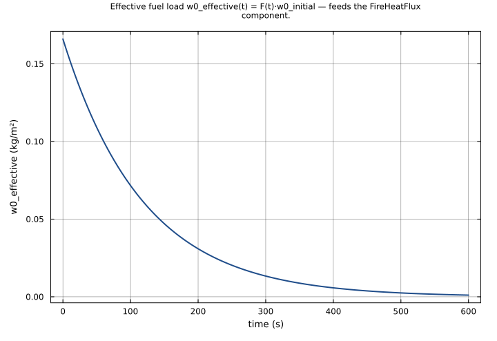
w0_effective = F * w0_initial (algebraic feedback to FireHeatFlux)
In the coupled WRF-SFIRE pipeline (couple2(LevelSetCoupler, FuelConsumptionCoupler) at coupling.jl:415), is_burning is driven by the level-set function via a smooth Heaviside is_burning = 0.5*(1 - tanh(ψ/ε_h)); when standalone, it stays a parameter and the user supplies a constant value. Likewise w0_initial and T_f are coupled from FuelModelLookup (coupling.jl:303) but default to free parameters here.
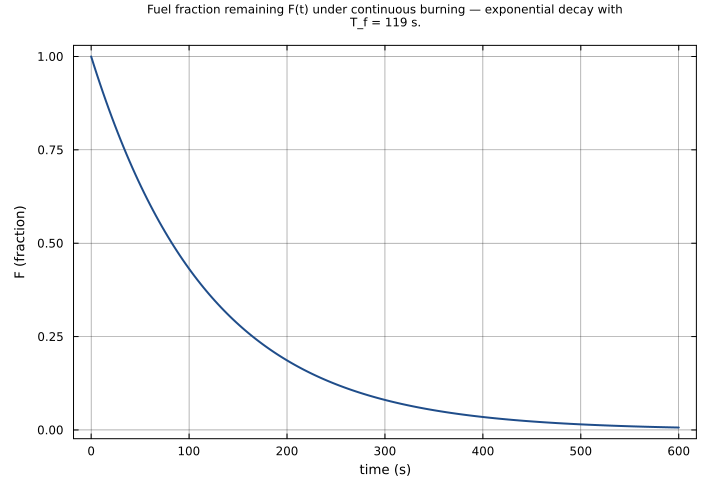
Analytical solution for constant is_burning: F(t) = exp(-is_burningt/T_f); w0_effective(t) = w0_initial * exp(-is_burningt/T_f). All inline tests below are evaluated against this closed form.
Tolerance rationale (model-level rel=1e-6): linear constant-coefficient scalar ODE; SciPy LSODA truncation is far below 1e-6 over the tested horizons (≤1200 s, ≤30 e-folding times kept ≤3). Algebraic w0_effective inherits the same accuracy since it is a single multiply on F. Tests use the default tolerance throughout — no per-test loosening needed._
Variables
| Name | Units | Default | Description |
|---|---|---|---|
F | 1 | 1.0 | Fuel fraction remaining (1=full, 0=consumed). |
Parameters
| Name | Units | Default | Description |
|---|---|---|---|
T_f | s | 119.0 | Fuel burn time constant (1/e decay time). Default 119 s ≈ 0.166 / 0.8514·166 (Anderson grass-fuel; T_f ≈ w / 0.8514·166 per Mandel et al. 2011). |
w0_initial | kg/m^2 | 0.166 | Initial oven-dry fuel load (Anderson 1982 fuel model 1 grass default). |
is_burning | 1 | 0.0 | Whether the fuel is burning (1=yes, 0=no, dimensionless). In the coupled level-set system this is driven by 0.5*(1 - tanh(ψ/ε_h)). |
Observed
| Name | Units | Default | Description |
|---|---|---|---|
w0_effective | kg/m^2 | Effective fuel load after consumption — feeds FireHeatFlux. |
Observed expressions
$$ w0_{effective} = F \cdot w0_{initial} $$Effective fuel load after consumption — feeds FireHeatFlux.
Equations
$$ \mathrm{D}\left(F\right) = \frac{\left(-1.0\right) \cdot is_{burning} \cdot F}{T_{f}} $$Analyses
anderson_grass_decay_curve
Anderson (1982) fuel model 1 grass: T_f=119 s, w0_initial=0.166 kg/m², continuous burning (is_burning=1). Reproduces the Mandel et al. (2011) Eq. 3 fuel-fraction decay curve over five e-folding times.
Time span: 0.0 → 600.0
is_burning_sweep
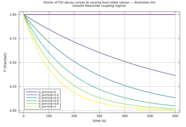
Sweep is_burning from 0 to 1 at fixed T_f and w0_initial, sampling the smoothed Heaviside values that the LevelSetFireSpread coupling produces. Surfaces the linear scaling of the effective decay constant (is_burning/T_f) on the F(t) curve.
Time span: 0.0 → 600.0
Swept over: is_burning
Raw .esm
Raw .esm JSON (this component)
{
  "reference": {
    "citation": "Mandel, J., Beezley, J.D., and Kochanski, A.K. (2011). Coupled atmosphere-wildland fire modeling with WRF 3.3 and SFIRE 2011. Geosci. Model Dev., 4, 591–610. doi:10.5194/gmd-4-591-2011.",
    "notes": "source_ref: WildlandFire.jl:src/level_set_fire_spread.jl:243\nUpstream `FuelConsumption` is an MTK `@component` with two `@variables` — F(t)=1.0 (fuel fraction remaining) and w0_effective(t) (algebraic) — and three `@parameters` (T_f, w0_initial, is_burning=0.0). The two equations are preserved verbatim:\n  D(F) = -is_burning * F / T_f                 (Eq. 3, Mandel et al. 2011, differential form)\n  w0_effective = F * w0_initial                 (algebraic feedback to FireHeatFlux)\n\nIn the coupled WRF-SFIRE pipeline (couple2(LevelSetCoupler, FuelConsumptionCoupler) at coupling.jl:415), is_burning is driven by the level-set function via a smooth Heaviside is_burning = 0.5*(1 - tanh(ψ/ε_h)); when standalone, it stays a parameter and the user supplies a constant value. Likewise w0_initial and T_f are coupled from FuelModelLookup (coupling.jl:303) but default to free parameters here.\n\nAnalytical solution for constant is_burning: F(t) = exp(-is_burning*t/T_f); w0_effective(t) = w0_initial * exp(-is_burning*t/T_f). All inline tests below are evaluated against this closed form.\n\nTolerance rationale (model-level rel=1e-6): linear constant-coefficient scalar ODE; SciPy LSODA truncation is far below 1e-6 over the tested horizons (≤1200 s, ≤30 e-folding times kept ≤3). Algebraic w0_effective inherits the same accuracy since it is a single multiply on F. Tests use the default tolerance throughout — no per-test loosening needed."
  },
  "tolerance": {
    "rel": 1e-06
  },
  "variables": {
    "T_f": {
      "type": "parameter",
      "units": "s",
      "default": 119.0,
      "description": "Fuel burn time constant (1/e decay time). Default 119 s ≈ 0.166 / 0.8514·166 (Anderson grass-fuel; T_f ≈ w / 0.8514·166 per Mandel et al. 2011)."
    },
    "w0_initial": {
      "type": "parameter",
      "units": "kg/m^2",
      "default": 0.166,
      "description": "Initial oven-dry fuel load (Anderson 1982 fuel model 1 grass default)."
    },
    "is_burning": {
      "type": "parameter",
      "units": "1",
      "default": 0.0,
      "description": "Whether the fuel is burning (1=yes, 0=no, dimensionless). In the coupled level-set system this is driven by 0.5*(1 - tanh(ψ/ε_h))."
    },
    "F": {
      "type": "unknown",
      "units": "1",
      "default": 1.0,
      "description": "Fuel fraction remaining (1=full, 0=consumed)."
    },
    "w0_effective": {
      "type": "unknown",
      "units": "kg/m^2",
      "description": "Effective fuel load after consumption — feeds FireHeatFlux."
    }
  },
  "equations": [
    {
      "lhs": {
        "op": "D",
        "wrt": "t",
        "args": [
          "F"
        ]
      },
      "rhs": {
        "op": "/",
        "args": [
          {
            "op": "*",
            "args": [
              -1.0,
              "is_burning",
              "F"
            ]
          },
          "T_f"
        ]
      }
    },
    {
      "lhs": "w0_effective",
      "rhs": {
        "op": "*",
        "args": [
          "F",
          "w0_initial"
        ]
      }
    }
  ],
  "tests": [
    {
      "id": "no_burning_F_constant",
      "description": "is_burning = 0 — fuel is unignited. The ODE collapses to D(F) = 0, so F stays at its initial value of 1.0 for all time. w0_effective = F·w0_initial stays at w0_initial. Sanity check that the multiplicative is_burning gate works.",
      "parameter_overrides": {
        "is_burning": 0.0,
        "T_f": 119.0,
        "w0_initial": 0.5
      },
      "initial_conditions": {
        "F": 1.0
      },
      "time_span": {
        "start": 0.0,
        "end": 1000.0
      },
      "assertions": [
        {
          "variable": "F",
          "time": 0.0,
          "expected": 1.0
        },
        {
          "variable": "F",
          "time": 500.0,
          "expected": 1.0
        },
        {
          "variable": "F",
          "time": 1000.0,
          "expected": 1.0
        },
        {
          "variable": "w0_effective",
          "time": 0.0,
          "expected": 0.5
        },
        {
          "variable": "w0_effective",
          "time": 1000.0,
          "expected": 0.5
        }
      ]
    },
    {
      "id": "anderson_grass_full_burn",
      "description": "Anderson (1982) fuel model 1 grass parameters with is_burning=1: T_f=119 s, w0_initial=0.166 kg/m². Closed-form F(t)=exp(-t/119); w0_effective(t)=0.166·exp(-t/119). Sample at t=0 (F=1, w0_eff=0.166), t=119 (F=exp(-1), w0_eff=0.166·exp(-1)), t=238 (F=exp(-2), w0_eff=0.166·exp(-2)).",
      "parameter_overrides": {
        "is_burning": 1.0,
        "T_f": 119.0,
        "w0_initial": 0.166
      },
      "initial_conditions": {
        "F": 1.0
      },
      "time_span": {
        "start": 0.0,
        "end": 238.0
      },
      "assertions": [
        {
          "variable": "F",
          "time": 0.0,
          "expected": 1.0
        },
        {
          "variable": "F",
          "time": 119.0,
          "expected": 0.36787944117144233
        },
        {
          "variable": "F",
          "time": 238.0,
          "expected": 0.1353352832366127
        },
        {
          "variable": "w0_effective",
          "time": 0.0,
          "expected": 0.166
        },
        {
          "variable": "w0_effective",
          "time": 119.0,
          "expected": 0.06106798723445943
        },
        {
          "variable": "w0_effective",
          "time": 238.0,
          "expected": 0.02246565701727771
        }
      ]
    },
    {
      "id": "partial_burning_state",
      "description": "Partial burning (is_burning=0.5) with T_f=200, w0_initial=1.0. The effective decay constant is is_burning/T_f = 1/400, so F(t)=exp(-t/400). Sample at t=0, t=400 (F=exp(-1)), t=800 (F=exp(-2)). Verifies that is_burning enters the decay rate multiplicatively, not as a binary gate.",
      "parameter_overrides": {
        "is_burning": 0.5,
        "T_f": 200.0,
        "w0_initial": 1.0
      },
      "initial_conditions": {
        "F": 1.0
      },
      "time_span": {
        "start": 0.0,
        "end": 800.0
      },
      "assertions": [
        {
          "variable": "F",
          "time": 0.0,
          "expected": 1.0
        },
        {
          "variable": "F",
          "time": 400.0,
          "expected": 0.36787944117144233
        },
        {
          "variable": "F",
          "time": 800.0,
          "expected": 0.1353352832366127
        },
        {
          "variable": "w0_effective",
          "time": 0.0,
          "expected": 1.0
        },
        {
          "variable": "w0_effective",
          "time": 400.0,
          "expected": 0.36787944117144233
        },
        {
          "variable": "w0_effective",
          "time": 800.0,
          "expected": 0.1353352832366127
        }
      ]
    },
    {
      "id": "fast_burn_short_T_f",
      "description": "Fast burn (T_f=10 s, is_burning=1, w0_initial=2.0): F drops to ~5% in three e-folding times. F(t)=exp(-t/10), w0_effective(t)=2·exp(-t/10). At t=10, F=exp(-1)≈0.368, w0_eff=2·exp(-1)≈0.736. At t=30, F=exp(-3)≈0.0498, w0_eff≈0.0996. Stress-test of the ODE integrator on a short-time-constant system.",
      "parameter_overrides": {
        "is_burning": 1.0,
        "T_f": 10.0,
        "w0_initial": 2.0
      },
      "initial_conditions": {
        "F": 1.0
      },
      "time_span": {
        "start": 0.0,
        "end": 30.0
      },
      "assertions": [
        {
          "variable": "F",
          "time": 0.0,
          "expected": 1.0
        },
        {
          "variable": "F",
          "time": 10.0,
          "expected": 0.36787944117144233
        },
        {
          "variable": "F",
          "time": 30.0,
          "expected": 0.049787068367863944
        },
        {
          "variable": "w0_effective",
          "time": 10.0,
          "expected": 0.7357588823428847
        },
        {
          "variable": "w0_effective",
          "time": 30.0,
          "expected": 0.09957413673572789
        }
      ]
    },
    {
      "id": "w0_effective_product_identity",
      "description": "Cross-check the product identity w0_effective ≡ F·w0_initial: pick is_burning=0.5, T_f=50, w0_initial=10.0, sample at t=50 where F=exp(-0.5·50/50)=exp(-0.5)≈0.6065 → w0_effective=6.0653. Verifies that the algebraic equation tracks the ODE state exactly (modulo float64 multiply roundoff).",
      "parameter_overrides": {
        "is_burning": 0.5,
        "T_f": 50.0,
        "w0_initial": 10.0
      },
      "initial_conditions": {
        "F": 1.0
      },
      "time_span": {
        "start": 0.0,
        "end": 50.0
      },
      "assertions": [
        {
          "variable": "F",
          "time": 50.0,
          "expected": 0.6065306597126334
        },
        {
          "variable": "w0_effective",
          "time": 50.0,
          "expected": 6.065306597126334
        }
      ]
    }
  ],
  "analyses": [
    {
      "id": "anderson_grass_decay_curve",
      "description": "Anderson (1982) fuel model 1 grass: T_f=119 s, w0_initial=0.166 kg/m², continuous burning (is_burning=1). Reproduces the Mandel et al. (2011) Eq. 3 fuel-fraction decay curve over five e-folding times.",
      "initial_state": {
        "F": 1.0
      },
      "parameters": {
        "is_burning": 1.0,
        "T_f": 119.0,
        "w0_initial": 0.166
      },
      "time_span": {
        "start": 0.0,
        "end": 600.0
      },
      "plots": [
        {
          "id": "F_vs_time",
          "type": "line",
          "description": "Fuel fraction remaining F(t) under continuous burning — exponential decay with T_f = 119 s.",
          "x": {
            "variable": "t",
            "label": "time (s)"
          },
          "y": {
            "variable": "F",
            "label": "F (fraction)"
          }
        },
        {
          "id": "w0_effective_vs_time",
          "type": "line",
          "description": "Effective fuel load w0_effective(t) = F(t)·w0_initial — feeds the FireHeatFlux component.",
          "x": {
            "variable": "t",
            "label": "time (s)"
          },
          "y": {
            "variable": "w0_effective",
            "label": "w0_effective (kg/m²)"
          }
        }
      ]
    },
    {
      "id": "is_burning_sweep",
      "description": "Sweep is_burning from 0 to 1 at fixed T_f and w0_initial, sampling the smoothed Heaviside values that the LevelSetFireSpread coupling produces. Surfaces the linear scaling of the effective decay constant (is_burning/T_f) on the F(t) curve.",
      "initial_state": {
        "F": 1.0
      },
      "parameters": {
        "T_f": 119.0,
        "w0_initial": 0.166
      },
      "time_span": {
        "start": 0.0,
        "end": 600.0
      },
      "parameter_sweep": {
        "type": "cartesian",
        "dimensions": [
          {
            "parameter": "is_burning",
            "range": {
              "start": 0.0,
              "stop": 1.0,
              "count": 6,
              "scale": "linear"
            }
          }
        ]
      },
      "plots": [
        {
          "id": "F_curves_vs_is_burning",
          "type": "line",
          "description": "Family of F(t) decay curves at varying burn-state values — illustrates the smooth-Heaviside coupling regime.",
          "x": {
            "variable": "t",
            "label": "time (s)"
          },
          "y": {
            "variable": "F",
            "label": "F (fraction)"
          }
        }
      ]
    }
  ]
}