HeatFlux
Vertical heat flux across the interface between two soil/snow/road/wall/roof layers via the finite-difference discretization of Fourier's law of heat conduction (Oleson et al. 2010 Eq. 4.11). Migrated from UrbanCanopy.jl@9200edd4 src/roof_wall_road_snow_temperatures.jl:312 (`HeatFlux` @component). Implements the canonical layer-pair flux F = -λ_interface * (T_i - T_{i+1}) / (z_{i+1} - z_i), positive upward (heat flowing from layer i+1 to layer i, i.e. from deeper layer to shallower layer when stacking depth-increasing-downward). λ_interface is the harmonic-mean interface conductivity (Eq. 4.12), produced upstream by InterfaceThermalConductivity from the adjacent-layer bulk conductivities. Parameterized as observed-only with one algebraic equation: F is the state variable; λ_interface, T_i, T_ip1, z_i, z_ip1 are inputs (parameters in standalone form, wired to upstream components in a full column build).
Description
Vertical heat flux across the interface between two soil/snow/road/wall/roof layers via the finite-difference discretization of Fourier’s law of heat conduction (Oleson et al. 2010 Eq. 4.11). Migrated from UrbanCanopy.jl@9200edd4 src/roof_wall_road_snow_temperatures.jl:312 (HeatFlux @component). Implements the canonical layer-pair flux F = -λ_interface * (T_i - T_{i+1}) / (z_{i+1} - z_i), positive upward (heat flowing from layer i+1 to layer i, i.e. from deeper layer to shallower layer when stacking depth-increasing-downward). λ_interface is the harmonic-mean interface conductivity (Eq. 4.12), produced upstream by InterfaceThermalConductivity from the adjacent-layer bulk conductivities. Parameterized as observed-only with one algebraic equation: F is the state variable; λ_interface, T_i, T_ip1, z_i, z_ip1 are inputs (parameters in standalone form, wired to upstream components in a full column build).
Reference
_source_ref: UrbanCanopy.jl@9200edd4f15609f20339d3a7d104de8064544310:src/roof_wall_road_snow_temperatures.jl:312
Upstream HeatFlux is an MTK @component with five @parameters (λ_interface, T_i, T_ip1, z_i, z_ip1), one time-indexed @variable (F), and one algebraic equation (Eq. 4.11 — no derivatives, no @constants). Identical equation structure preserved here. Upstream canonical test (test/roof_wall_road_snow_temperatures_test.jl:250) drives the equation through mtkcompile + ODEProblem + solve and asserts the flux value, sign, and zero-gradient limit; that fixture is reproduced verbatim here as the upstream_equation_verification and upstream_equal_temperatures_zero_flux test pair.
The upstream HeatFlux is the layer-pair building block of CLMU’s column heat-conduction discretization (Oleson Section 4.1). Within a full column build, λ_interface comes from the upstream InterfaceThermalConductivity component (Eq. 4.12 harmonic-mean of adjacent-layer bulk conductivities), z_i and z_ip1 are node depths from the column geometry components (SnowLayerGeometry, UniformGrid, ExponentialGrid), T_i and T_ip1 are state variables from the column’s per-layer temperature ODE. In standalone form (this ESM), all five are exposed as @parameters, allowing the algebraic Eq. 4.11 to be exercised directly without wiring the rest of the column.
Unicode parameter name: λ_interface is preserved from upstream — peer ESM components in this rig (snow_melt_no_layers.esm uses Δt, freezing_point_depression.esm uses Δz/θ_sat/ψ_sat/ρ_liq, snow_density.esm uses ρ_*) already use unicode in identifiers and the schema’s identifier pattern allows it. λ_interface is an @parameters input (not an @constants), matching the freezing_point_depression convention rather than the surface_energy_flux convention of ASCII-renaming @constants (σ_SB → sigma_SB, ε_g → epsilon_g) since there are no @constants in this component.
Sign convention: F is positive upward — i.e. heat flowing from the deeper layer (i+1) into the shallower layer (i) when the column is depth-increasing-downward (z_ip1 > z_i, the standard CLMU convention). The leading minus in Eq. 4.11 captures Fourier’s law F = -λ ∇T (heat flows from hot to cold), so when T_i > T_ip1 (shallower hotter than deeper, the typical daytime forcing under solar heating of the surface) F = -λ * (positive)/(positive) is negative — i.e. heat is flowing downward into the column (away from the surface). When T_i < T_ip1 (shallower colder than deeper, e.g. radiative cooling of the surface at night), F is positive — heat is flowing upward from the warmer subsurface into the cold near-surface layer. The upstream test (test/roof_wall_road_snow_temperatures_test.jl:265) asserts F < 0 for T_i = 300 > T_ip1 = 290 to anchor this sign convention; the migrated upstream_equation_verification test reproduces the expected F = -100 W/m^2 numeric value at rtol = 1e-10.
Equation form: the upstream -λ_interface * (T_i - T_ip1) / (z_ip1 - z_i) form is preserved verbatim in the AST. The leading unary minus is encoded as (0 - λ_interface) per the convention used by surface_energy_flux.esm (its dh_dT = -dL_g_dT - ... term uses {op:-, args:[0, dL_g_dT]} for the leading negation). Mathematically equivalent to the algebraically-equivalent rewrite λ_interface * (T_ip1 - T_i) / (z_ip1 - z_i) (which only uses binary subtraction), but the verbatim form preserves the docstring’s direct correspondence to the canonical Fourier’s law form F = -λ * dT/dz so a reviewer sees the same algebraic shape in the ESM AST as in the upstream Julia source. Arithmetically identical to the rewrite at IEEE-754 ULP precision for all finite inputs.
Observability classification: this component is functionally observed-only — the single output variable F is given by a single algebraic equation in the five parameters (the (t) time index has no role since there is no derivative). Test scenarios use time_span: [0, 1] and sample at t=0 to mirror the convention used by sibling observed-only ESM files in this rig (heating_cooling_flux.esm, snow_melt_no_layers.esm, total_phase_change_energy.esm, freezing_point_depression.esm).
Tolerance rationale (model-level rel=1e-9): observed-only single-equation algebraic system (no ODE integration); Eq. 4.11 evaluates as one multiplication, one subtraction (numerator difference), one subtraction (denominator difference), and one division — all at IEEE-754 ULP precision (~1e-16). 1e-9 leaves comfortable headroom above ULP roundoff and matches the convention used by sibling observed-only files in this rig (total_phase_change_energy.esm and heating_cooling_flux.esm both use 1e-9). Tighter abs: 1e-12 is asserted on outputs that are exactly zero by construction (equal-temperatures limit, zero-conductivity limit) so the assertion does not silently accept a stuck-at-1e-3 regression.
Upstream tolerance reproduction: the upstream canonical test uses rtol = 1.0e-10 on the F ≈ -100 assertion and atol = 1.0e-12 on the F ≈ 0 equal-temperatures assertion. Re-asserted at the same tolerances via per-assertion tolerance blocks on the upstream-canonical tests, tighter than the model-level default for the F = -100 assertion._
Parameters
| Name | Units | Default | Description |
|---|---|---|---|
λ_interface | W/(m*K) | 1.0 | Thermal conductivity at the interface between layers i and i+1 (Oleson Eq. 4.12) — harmonic mean of adjacent-layer bulk conductivities; produced upstream by InterfaceThermalConductivity in a full column build, exposed as an input parameter in standalone form |
T_i | K | 300.0 | Temperature of layer i (the shallower layer when depth-increasing-downward); upstream a state variable from the column-temperature ODE, exposed as an input parameter in standalone form |
T_ip1 | K | 290.0 | Temperature of layer i+1 (the deeper layer when depth-increasing-downward); upstream a state variable from the column-temperature ODE, exposed as an input parameter in standalone form |
z_i | m | 0.05 | Node depth of layer i (positive downward by CLMU convention); upstream from the column geometry components (SnowLayerGeometry / UniformGrid / ExponentialGrid) |
z_ip1 | m | 0.15 | Node depth of layer i+1 (positive downward by CLMU convention; z_ip1 > z_i); upstream from the column geometry components |
Observed
| Name | Units | Default | Description |
|---|---|---|---|
F | W/m^2 | Heat flux from layer i+1 to layer i across the interface (Oleson Eq. 4.11), positive upward: F = -λ_interface * (T_i - T_ip1) / (z_ip1 - z_i); negative under daytime downward-conduction forcing (T_i > T_ip1), positive under nighttime upward-conduction forcing (T_i < T_ip1) |
Observed expressions
$$ F = \frac{\left(0.0 - λ_{interface}\right) \cdot \left(T_{i} - T_{ip1}\right)}{z_{ip1} - z_{i}} $$Heat flux from layer i+1 to layer i across the interface (Oleson Eq. 4.11), positive upward: F = -λ_interface * (T_i - T_ip1) / (z_ip1 - z_i); negative under daytime downward-conduction forcing (T_i > T_ip1), positive under nighttime upward-conduction forcing (T_i < T_ip1)
Analyses
flux_vs_temperature_difference
Sweep T_i across a 100 K range (240 K to 340 K) at fixed T_ip1 = 290 K, λ_interface = 1.0, z_i = 0.05, z_ip1 = 0.15. Surfaces the linear F = -λ * (T_i - T_ip1) / dz response of Eq. 4.11: F passes through zero at T_i = T_ip1 = 290 K (the no-gradient point), is positive for T_i < T_ip1 (upward flux from warmer subsurface), and is negative for T_i > T_ip1 (downward flux from warmer surface). Slope -10 W/(m^2*K) (= -λ/dz). The canonical Fourier-law line plot.
Time span: 0.0 → 1.0
Swept over: T_i
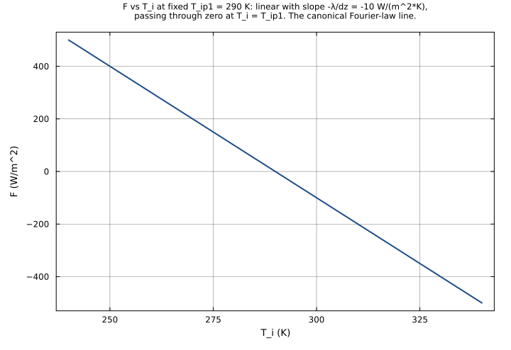
flux_vs_layer_spacing
Sweep z_ip1 across a 0.02-2 m range at fixed z_i = 0.0, λ_interface = 1.0, T_i = 300 K, T_ip1 = 290 K → F = -1.0 * 10 / z_ip1 = -10 / z_ip1. Surfaces the 1/dz hyperbolic dependence of conductive flux on layer spacing: thin layers carry huge fluxes, thick layers carry small fluxes. The high-flux corner at z_ip1 → 0.02 (small dz) is the regime that motivates the use of finer near-surface grids in CLMU; the asymptotic low-flux tail at large dz is the deep-soil regime.
Time span: 0.0 → 1.0
Swept over: z_ip1
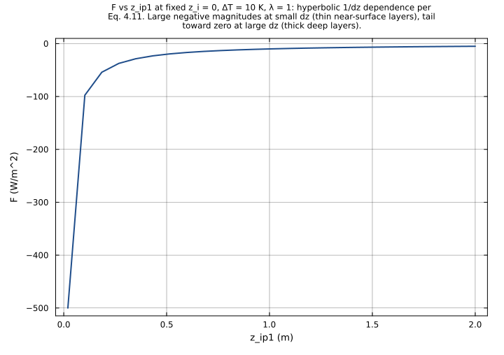
flux_heatmap_lambda_vs_dT
2D heatmap surfacing the joint dependence of F on λ_interface and the temperature difference (T_i - T_ip1). Sweep λ_interface across a realistic CLMU range (0.1 W/(mK) for snow → 3 W/(mK) for moist soil / concrete) and T_i over a 100 K range at fixed T_ip1 = 290 K, z_i = 0.05 m, z_ip1 = 0.15 m. The surface F = -λ * (T_i - 290) / 0.1 is a bilinear function of (λ, T_i); iso-flux contours are hyperbolic lines in (λ, T_i) space. The horizontal line T_i = 290 K is the zero-flux ridge; below it F > 0 (upward, blue), above F < 0 (downward, red).
Time span: 0.0 → 1.0
Swept over: λ_interface, T_i
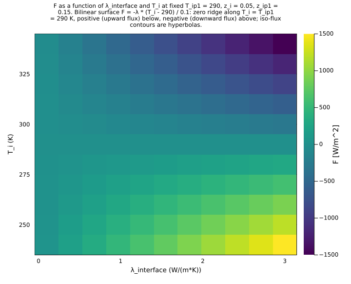
Raw .esm
Raw .esm JSON (this component)
{
  "reference": {
    "notes": "source_ref: UrbanCanopy.jl@9200edd4f15609f20339d3a7d104de8064544310:src/roof_wall_road_snow_temperatures.jl:312\nUpstream `HeatFlux` is an MTK `@component` with five `@parameters` (λ_interface, T_i, T_ip1, z_i, z_ip1), one time-indexed `@variable` (F), and one algebraic equation (Eq. 4.11 — no derivatives, no `@constants`). Identical equation structure preserved here. Upstream canonical test (test/roof_wall_road_snow_temperatures_test.jl:250) drives the equation through `mtkcompile` + `ODEProblem` + `solve` and asserts the flux value, sign, and zero-gradient limit; that fixture is reproduced verbatim here as the `upstream_equation_verification` and `upstream_equal_temperatures_zero_flux` test pair.\n\nThe upstream `HeatFlux` is the layer-pair building block of CLMU's column heat-conduction discretization (Oleson Section 4.1). Within a full column build, λ_interface comes from the upstream `InterfaceThermalConductivity` component (Eq. 4.12 harmonic-mean of adjacent-layer bulk conductivities), z_i and z_ip1 are node depths from the column geometry components (`SnowLayerGeometry`, `UniformGrid`, `ExponentialGrid`), T_i and T_ip1 are state variables from the column's per-layer temperature ODE. In standalone form (this ESM), all five are exposed as `@parameters`, allowing the algebraic Eq. 4.11 to be exercised directly without wiring the rest of the column.\n\nUnicode parameter name: `λ_interface` is preserved from upstream — peer ESM components in this rig (snow_melt_no_layers.esm uses Δt, freezing_point_depression.esm uses Δz/θ_sat/ψ_sat/ρ_liq, snow_density.esm uses ρ_*) already use unicode in identifiers and the schema's identifier pattern allows it. λ_interface is an `@parameters` input (not an `@constants`), matching the freezing_point_depression convention rather than the surface_energy_flux convention of ASCII-renaming `@constants` (σ_SB → sigma_SB, ε_g → epsilon_g) since there are no `@constants` in this component.\n\nSign convention: F is positive upward — i.e. heat flowing from the deeper layer (i+1) into the shallower layer (i) when the column is depth-increasing-downward (z_ip1 > z_i, the standard CLMU convention). The leading minus in Eq. 4.11 captures Fourier's law `F = -λ ∇T` (heat flows from hot to cold), so when T_i > T_ip1 (shallower hotter than deeper, the typical daytime forcing under solar heating of the surface) F = -λ * (positive)/(positive) is **negative** — i.e. heat is flowing downward into the column (away from the surface). When T_i < T_ip1 (shallower colder than deeper, e.g. radiative cooling of the surface at night), F is **positive** — heat is flowing upward from the warmer subsurface into the cold near-surface layer. The upstream test (test/roof_wall_road_snow_temperatures_test.jl:265) asserts F < 0 for T_i = 300 > T_ip1 = 290 to anchor this sign convention; the migrated `upstream_equation_verification` test reproduces the expected F = -100 W/m^2 numeric value at rtol = 1e-10.\n\nEquation form: the upstream `-λ_interface * (T_i - T_ip1) / (z_ip1 - z_i)` form is preserved verbatim in the AST. The leading unary minus is encoded as `(0 - λ_interface)` per the convention used by surface_energy_flux.esm (its `dh_dT = -dL_g_dT - ...` term uses `{op:-, args:[0, dL_g_dT]}` for the leading negation). Mathematically equivalent to the algebraically-equivalent rewrite `λ_interface * (T_ip1 - T_i) / (z_ip1 - z_i)` (which only uses binary subtraction), but the verbatim form preserves the docstring's direct correspondence to the canonical Fourier's law form `F = -λ * dT/dz` so a reviewer sees the same algebraic shape in the ESM AST as in the upstream Julia source. Arithmetically identical to the rewrite at IEEE-754 ULP precision for all finite inputs.\n\nObservability classification: this component is functionally observed-only — the single output variable F is given by a single algebraic equation in the five parameters (the `(t)` time index has no role since there is no derivative). Test scenarios use `time_span: [0, 1]` and sample at t=0 to mirror the convention used by sibling observed-only ESM files in this rig (heating_cooling_flux.esm, snow_melt_no_layers.esm, total_phase_change_energy.esm, freezing_point_depression.esm).\n\nTolerance rationale (model-level rel=1e-9): observed-only single-equation algebraic system (no ODE integration); Eq. 4.11 evaluates as one multiplication, one subtraction (numerator difference), one subtraction (denominator difference), and one division — all at IEEE-754 ULP precision (~1e-16). 1e-9 leaves comfortable headroom above ULP roundoff and matches the convention used by sibling observed-only files in this rig (total_phase_change_energy.esm and heating_cooling_flux.esm both use 1e-9). Tighter `abs: 1e-12` is asserted on outputs that are exactly zero by construction (equal-temperatures limit, zero-conductivity limit) so the assertion does not silently accept a stuck-at-1e-3 regression.\n\nUpstream tolerance reproduction: the upstream canonical test uses `rtol = 1.0e-10` on the F ≈ -100 assertion and `atol = 1.0e-12` on the F ≈ 0 equal-temperatures assertion. Re-asserted at the same tolerances via per-assertion `tolerance` blocks on the upstream-canonical tests, tighter than the model-level default for the F = -100 assertion."
  },
  "tolerance": {
    "rel": 1e-09
  },
  "variables": {
    "λ_interface": {
      "type": "parameter",
      "units": "W/(m*K)",
      "default": 1.0,
      "description": "Thermal conductivity at the interface between layers i and i+1 (Oleson Eq. 4.12) — harmonic mean of adjacent-layer bulk conductivities; produced upstream by InterfaceThermalConductivity in a full column build, exposed as an input parameter in standalone form"
    },
    "T_i": {
      "type": "parameter",
      "units": "K",
      "default": 300.0,
      "description": "Temperature of layer i (the shallower layer when depth-increasing-downward); upstream a state variable from the column-temperature ODE, exposed as an input parameter in standalone form"
    },
    "T_ip1": {
      "type": "parameter",
      "units": "K",
      "default": 290.0,
      "description": "Temperature of layer i+1 (the deeper layer when depth-increasing-downward); upstream a state variable from the column-temperature ODE, exposed as an input parameter in standalone form"
    },
    "z_i": {
      "type": "parameter",
      "units": "m",
      "default": 0.05,
      "description": "Node depth of layer i (positive downward by CLMU convention); upstream from the column geometry components (SnowLayerGeometry / UniformGrid / ExponentialGrid)"
    },
    "z_ip1": {
      "type": "parameter",
      "units": "m",
      "default": 0.15,
      "description": "Node depth of layer i+1 (positive downward by CLMU convention; z_ip1 > z_i); upstream from the column geometry components"
    },
    "F": {
      "type": "unknown",
      "units": "W/m^2",
      "description": "Heat flux from layer i+1 to layer i across the interface (Oleson Eq. 4.11), positive upward: F = -λ_interface * (T_i - T_ip1) / (z_ip1 - z_i); negative under daytime downward-conduction forcing (T_i > T_ip1), positive under nighttime upward-conduction forcing (T_i < T_ip1)"
    }
  },
  "equations": [
    {
      "lhs": "F",
      "rhs": {
        "op": "/",
        "args": [
          {
            "op": "*",
            "args": [
              {
                "op": "-",
                "args": [
                  0.0,
                  "λ_interface"
                ]
              },
              {
                "op": "-",
                "args": [
                  "T_i",
                  "T_ip1"
                ]
              }
            ]
          },
          {
            "op": "-",
            "args": [
              "z_ip1",
              "z_i"
            ]
          }
        ]
      }
    }
  ],
  "tests": [
    {
      "id": "upstream_equation_verification",
      "description": "Reproduces upstream `HeatFlux - Direction and Magnitude` test, first assertion (UrbanCanopy.jl test/roof_wall_road_snow_temperatures_test.jl:264). λ_interface = 1.0 W/(m*K), T_i = 300 K, T_ip1 = 290 K, z_i = 0.05 m, z_ip1 = 0.15 m → F = -1.0 * (300 - 290) / (0.15 - 0.05) = -100.0 W/m^2. The negative sign anchors the Fourier's-law convention (heat flowing downward into the column when the surface is hotter than the subsurface). Asserted at rtol = 1e-10 per the upstream test's stated tolerance.",
      "parameter_overrides": {
        "λ_interface": 1.0,
        "T_i": 300.0,
        "T_ip1": 290.0,
        "z_i": 0.05,
        "z_ip1": 0.15
      },
      "time_span": {
        "start": 0.0,
        "end": 1.0
      },
      "assertions": [
        {
          "variable": "F",
          "time": 0.0,
          "expected": -100.0,
          "tolerance": {
            "rel": 1e-10
          }
        }
      ]
    },
    {
      "id": "upstream_equal_temperatures_zero_flux",
      "description": "Reproduces upstream `HeatFlux - Direction and Magnitude` test, second assertion (UrbanCanopy.jl test/roof_wall_road_snow_temperatures_test.jl:275). Equal layer temperatures T_i = T_ip1 = 300 K → ΔT = 0 → F = 0 W/m^2 exactly. The other parameters (λ_interface, z_i, z_ip1) are held at the same values as `upstream_equation_verification` so this isolates the zero-gradient limit. Asserted at atol = 1e-12 per the upstream test's stated tolerance.",
      "parameter_overrides": {
        "λ_interface": 1.0,
        "T_i": 300.0,
        "T_ip1": 300.0,
        "z_i": 0.05,
        "z_ip1": 0.15
      },
      "time_span": {
        "start": 0.0,
        "end": 1.0
      },
      "assertions": [
        {
          "variable": "F",
          "time": 0.0,
          "expected": 0.0,
          "tolerance": {
            "abs": 1e-12
          }
        }
      ]
    },
    {
      "id": "reversed_gradient_positive_flux",
      "description": "Nighttime / radiative-cooling regime: T_i = 280 K (cold surface layer) < T_ip1 = 300 K (warm subsurface). λ_interface = 1.0, z_i = 0.05, z_ip1 = 0.15 → F = -1.0 * (280 - 300) / (0.15 - 0.05) = -1.0 * (-20) / 0.1 = +200.0 W/m^2. The positive sign confirms upward heat conduction when the subsurface is warmer than the surface (the inverse of the daytime case). Pins the sign convention against an accidental sign-flip in the migration.",
      "parameter_overrides": {
        "λ_interface": 1.0,
        "T_i": 280.0,
        "T_ip1": 300.0,
        "z_i": 0.05,
        "z_ip1": 0.15
      },
      "time_span": {
        "start": 0.0,
        "end": 1.0
      },
      "assertions": [
        {
          "variable": "F",
          "time": 0.0,
          "expected": 200.0
        }
      ]
    },
    {
      "id": "zero_conductivity_zero_flux",
      "description": "Insulator limit: λ_interface = 0 (no heat can cross the interface, e.g. a perfect insulating barrier). T_i = 300, T_ip1 = 250 with a strong 50 K gradient and small dz = 0.1 m — without insulation, F would be -500 W/m^2. With λ_interface = 0, F must be exactly zero (the multiplicative coefficient kills the entire RHS). Verifies the equation degenerates correctly in the zero-conductivity limit and exercises the multiplicative-zero path through the AST.",
      "parameter_overrides": {
        "λ_interface": 0.0,
        "T_i": 300.0,
        "T_ip1": 250.0,
        "z_i": 0.05,
        "z_ip1": 0.15
      },
      "time_span": {
        "start": 0.0,
        "end": 1.0
      },
      "assertions": [
        {
          "variable": "F",
          "time": 0.0,
          "expected": 0.0,
          "tolerance": {
            "abs": 1e-12
          }
        }
      ]
    },
    {
      "id": "unit_fourier_canonical",
      "description": "Canonical-units Fourier's-law sanity check: λ_interface = 1 W/(m*K), 1 K temperature drop over 1 m spacing → F = -1 * 1 / 1 = -1 W/m^2 exactly. The simplest possible non-degenerate input set; anchors that the multiplication and division are not accidentally swapped (e.g. dividing temperature by conductivity rather than multiplying) and that the layer-spacing denominator uses (z_ip1 - z_i) not (z_i - z_ip1).",
      "parameter_overrides": {
        "λ_interface": 1.0,
        "T_i": 1.0,
        "T_ip1": 0.0,
        "z_i": 0.0,
        "z_ip1": 1.0
      },
      "time_span": {
        "start": 0.0,
        "end": 1.0
      },
      "assertions": [
        {
          "variable": "F",
          "time": 0.0,
          "expected": -1.0
        }
      ]
    },
    {
      "id": "thin_layer_high_flux",
      "description": "Thin-layer regime: small dz = 0.01 m (1 cm spacing, typical of the thin top snow layer or the surface-skin layer of a road slab) with a moderate 10 K gradient and λ_interface = 1.5 → F = -1.5 * 10 / 0.01 = -1500 W/m^2. Magnitude one-and-a-half orders of magnitude above the baseline case, exercising the 1/dz hyperbolic scaling of the flux and confirming no precision loss at small denominators.",
      "parameter_overrides": {
        "λ_interface": 1.5,
        "T_i": 295.0,
        "T_ip1": 285.0,
        "z_i": 0.1,
        "z_ip1": 0.11
      },
      "time_span": {
        "start": 0.0,
        "end": 1.0
      },
      "assertions": [
        {
          "variable": "F",
          "time": 0.0,
          "expected": -1500.0
        }
      ]
    },
    {
      "id": "thick_layer_low_flux",
      "description": "Thick-layer regime: large dz = 2.0 m (typical of the deepest soil layer in a CLMU column) with a moderate 10 K gradient and λ_interface = 1.0 → F = -1.0 * 10 / 2.0 = -5.0 W/m^2. Magnitude two orders of magnitude below the baseline thin-layer case; exercises the small-flux end of the 1/dz scaling. The realistic regime in which the deep-soil layers carry only minor diffusive flux over the diurnal cycle.",
      "parameter_overrides": {
        "λ_interface": 1.0,
        "T_i": 290.0,
        "T_ip1": 280.0,
        "z_i": 1.0,
        "z_ip1": 3.0
      },
      "time_span": {
        "start": 0.0,
        "end": 1.0
      },
      "assertions": [
        {
          "variable": "F",
          "time": 0.0,
          "expected": -5.0
        }
      ]
    },
    {
      "id": "snow_layer_cold_regime",
      "description": "Winter sub-snow regime: both layer temperatures below freezing — T_i = 263.15 K (-10°C snow surface), T_ip1 = 268.15 K (-5°C deeper snow). Low snow thermal conductivity λ_interface = 0.4 W/(m*K) (typical bulk snow conductivity per Oleson Table 4.1), thin layer spacing dz = 0.05 m → F = -0.4 * (-5) / 0.05 = +40.0 W/m^2. Positive sign confirms upward conduction (warmer deeper snow heating the colder near-surface snow); realistic magnitude for the nocturnal winter heat-balance regime. Exercises the cold-regime / low-conductivity corner with a sign-flipped gradient.",
      "parameter_overrides": {
        "λ_interface": 0.4,
        "T_i": 263.15,
        "T_ip1": 268.15,
        "z_i": 0.025,
        "z_ip1": 0.075
      },
      "time_span": {
        "start": 0.0,
        "end": 1.0
      },
      "assertions": [
        {
          "variable": "F",
          "time": 0.0,
          "expected": 40.0
        }
      ]
    },
    {
      "id": "high_conductivity_road_slab",
      "description": "Road-slab regime: high thermal conductivity λ_interface = 2.5 W/(m*K) (concrete/asphalt, Oleson Table 4.1), small ΔT = 4 K, dz = 0.20 m → F = -2.5 * 4 / 0.20 = -50.0 W/m^2. Realistic mid-day heat flux into a heated concrete road slab. Exercises the high-λ corner balanced by a small gradient and moderate spacing.",
      "parameter_overrides": {
        "λ_interface": 2.5,
        "T_i": 310.0,
        "T_ip1": 306.0,
        "z_i": 0.1,
        "z_ip1": 0.3
      },
      "time_span": {
        "start": 0.0,
        "end": 1.0
      },
      "assertions": [
        {
          "variable": "F",
          "time": 0.0,
          "expected": -50.0
        }
      ]
    },
    {
      "id": "extreme_gradient_stress",
      "description": "Stress-test the high-flux corner: extreme 100 K gradient (representative of the surface-skin layer transition during peak insolation onto a sub-freezing snow surface), thin dz = 0.01 m, moderate λ_interface = 1.0 → F = -1.0 * 100 / 0.01 = -10000 W/m^2. Order-of-magnitude above any realistic CLMU column flux; confirms no numerical issues (overflow, loss of precision) in the high-magnitude corner of the parameter space.",
      "parameter_overrides": {
        "λ_interface": 1.0,
        "T_i": 350.0,
        "T_ip1": 250.0,
        "z_i": 0.1,
        "z_ip1": 0.11
      },
      "time_span": {
        "start": 0.0,
        "end": 1.0
      },
      "assertions": [
        {
          "variable": "F",
          "time": 0.0,
          "expected": -10000.0
        }
      ]
    },
    {
      "id": "zero_gradient_with_high_conductivity",
      "description": "Zero-gradient limit at high conductivity: T_i = T_ip1 = 290 K but with high λ_interface = 5.0 W/(m*K) — confirms that the zero-gradient flux is exactly zero regardless of how conductive the interface is (the multiplicative-zero through the numerator pins F = 0). Complements `upstream_equal_temperatures_zero_flux` (low λ, equal T) by varying λ; together they isolate the (T_i - T_ip1) factor as the sole driver of F = 0 in the equal-temperature limit.",
      "parameter_overrides": {
        "λ_interface": 5.0,
        "T_i": 290.0,
        "T_ip1": 290.0,
        "z_i": 0.05,
        "z_ip1": 0.15
      },
      "time_span": {
        "start": 0.0,
        "end": 1.0
      },
      "assertions": [
        {
          "variable": "F",
          "time": 0.0,
          "expected": 0.0,
          "tolerance": {
            "abs": 1e-12
          }
        }
      ]
    }
  ],
  "analyses": [
    {
      "id": "flux_vs_temperature_difference",
      "description": "Sweep T_i across a 100 K range (240 K to 340 K) at fixed T_ip1 = 290 K, λ_interface = 1.0, z_i = 0.05, z_ip1 = 0.15. Surfaces the linear F = -λ * (T_i - T_ip1) / dz response of Eq. 4.11: F passes through zero at T_i = T_ip1 = 290 K (the no-gradient point), is positive for T_i < T_ip1 (upward flux from warmer subsurface), and is negative for T_i > T_ip1 (downward flux from warmer surface). Slope -10 W/(m^2*K) (= -λ/dz). The canonical Fourier-law line plot.",
      "initial_state": {},
      "parameters": {
        "λ_interface": 1.0,
        "T_ip1": 290.0,
        "z_i": 0.05,
        "z_ip1": 0.15
      },
      "time_span": {
        "start": 0.0,
        "end": 1.0
      },
      "parameter_sweep": {
        "type": "cartesian",
        "dimensions": [
          {
            "parameter": "T_i",
            "range": {
              "start": 240.0,
              "stop": 340.0,
              "count": 21,
              "scale": "linear"
            }
          }
        ]
      },
      "plots": [
        {
          "id": "F_vs_T_i_line",
          "type": "line",
          "description": "F vs T_i at fixed T_ip1 = 290 K: linear with slope -λ/dz = -10 W/(m^2*K), passing through zero at T_i = T_ip1. The canonical Fourier-law line.",
          "x": {
            "variable": "T_i",
            "label": "T_i (K)"
          },
          "y": {
            "variable": "F",
            "label": "F (W/m^2)"
          }
        }
      ]
    },
    {
      "id": "flux_vs_layer_spacing",
      "description": "Sweep z_ip1 across a 0.02-2 m range at fixed z_i = 0.0, λ_interface = 1.0, T_i = 300 K, T_ip1 = 290 K → F = -1.0 * 10 / z_ip1 = -10 / z_ip1. Surfaces the 1/dz hyperbolic dependence of conductive flux on layer spacing: thin layers carry huge fluxes, thick layers carry small fluxes. The high-flux corner at z_ip1 → 0.02 (small dz) is the regime that motivates the use of finer near-surface grids in CLMU; the asymptotic low-flux tail at large dz is the deep-soil regime.",
      "initial_state": {},
      "parameters": {
        "λ_interface": 1.0,
        "T_i": 300.0,
        "T_ip1": 290.0,
        "z_i": 0.0
      },
      "time_span": {
        "start": 0.0,
        "end": 1.0
      },
      "parameter_sweep": {
        "type": "cartesian",
        "dimensions": [
          {
            "parameter": "z_ip1",
            "range": {
              "start": 0.02,
              "stop": 2.0,
              "count": 25,
              "scale": "linear"
            }
          }
        ]
      },
      "plots": [
        {
          "id": "F_vs_z_ip1_line",
          "type": "line",
          "description": "F vs z_ip1 at fixed z_i = 0, ΔT = 10 K, λ = 1: hyperbolic 1/dz dependence per Eq. 4.11. Large negative magnitudes at small dz (thin near-surface layers), tail toward zero at large dz (thick deep layers).",
          "x": {
            "variable": "z_ip1",
            "label": "z_ip1 (m)"
          },
          "y": {
            "variable": "F",
            "label": "F (W/m^2)"
          }
        }
      ]
    },
    {
      "id": "flux_heatmap_lambda_vs_dT",
      "description": "2D heatmap surfacing the joint dependence of F on λ_interface and the temperature difference (T_i - T_ip1). Sweep λ_interface across a realistic CLMU range (0.1 W/(m*K) for snow → 3 W/(m*K) for moist soil / concrete) and T_i over a 100 K range at fixed T_ip1 = 290 K, z_i = 0.05 m, z_ip1 = 0.15 m. The surface F = -λ * (T_i - 290) / 0.1 is a bilinear function of (λ, T_i); iso-flux contours are hyperbolic lines in (λ, T_i) space. The horizontal line T_i = 290 K is the zero-flux ridge; below it F > 0 (upward, blue), above F < 0 (downward, red).",
      "initial_state": {},
      "parameters": {
        "T_ip1": 290.0,
        "z_i": 0.05,
        "z_ip1": 0.15
      },
      "time_span": {
        "start": 0.0,
        "end": 1.0
      },
      "parameter_sweep": {
        "type": "cartesian",
        "dimensions": [
          {
            "parameter": "λ_interface",
            "range": {
              "start": 0.1,
              "stop": 3.0,
              "count": 11,
              "scale": "linear"
            }
          },
          {
            "parameter": "T_i",
            "range": {
              "start": 240.0,
              "stop": 340.0,
              "count": 11,
              "scale": "linear"
            }
          }
        ]
      },
      "plots": [
        {
          "id": "F_heatmap",
          "type": "heatmap",
          "description": "F as a function of λ_interface and T_i at fixed T_ip1 = 290, z_i = 0.05, z_ip1 = 0.15. Bilinear surface F = -λ * (T_i - 290) / 0.1: zero ridge along T_i = T_ip1 = 290 K, positive (upward flux) below, negative (downward flux) above; iso-flux contours are hyperbolas.",
          "x": {
            "variable": "λ_interface",
            "label": "λ_interface (W/(m*K))"
          },
          "y": {
            "variable": "T_i",
            "label": "T_i (K)"
          },
          "value": {
            "variable": "F",
            "reduce": "final"
          }
        }
      ]
    }
  ]
}