CLMUAtmosphere
Atmospheric interface for the Community Land Model Urban (CLMU) parameterization, following Chapter 1 of Oleson et al. (2010). Computes three diagnostic outputs from atmospheric forcing inputs: atmospheric vapor pressure (e_atm = q_atm P_atm / (epsilon + (1-epsilon) q_atm)), atmospheric air density (rho_atm = (P_atm - (1-epsilon) e_atm) / (R_da T_atm)), and the reference height for flux computations (z_atm = z_prime_atm + z_0 + z_d). Here epsilon = MW_wv/MW_da = 0.622 is the molecular-weight ratio of water vapor to dry air, and R_da = R_gas/MW_da is the specific gas constant for dry air. The urban canyon is represented as a roof + sunlit/shaded wall + pervious/impervious road five-column system; this component defines the atmospheric forcing interface that the rest of the canopy column reads. Migrated from UrbanCanopy.jl@9200edd4 src/clmu_introduction.jl:22 (`CLMUAtmosphere` @component). Parameterized as observed-only: forcings (q_atm, P_atm, T_atm, z_prime_atm, z_0, z_d, etc.) are inputs (parameters); e_atm, rho_atm, z_atm are the algebraic state outputs.
Description
Atmospheric interface for the Community Land Model Urban (CLMU) parameterization, following Chapter 1 of Oleson et al. (2010). Computes three diagnostic outputs from atmospheric forcing inputs: atmospheric vapor pressure (e_atm = q_atm P_atm / (epsilon + (1-epsilon) q_atm)), atmospheric air density (rho_atm = (P_atm - (1-epsilon) e_atm) / (R_da T_atm)), and the reference height for flux computations (z_atm = z_prime_atm + z_0 + z_d). Here epsilon = MW_wv/MW_da = 0.622 is the molecular-weight ratio of water vapor to dry air, and R_da = R_gas/MW_da is the specific gas constant for dry air. The urban canyon is represented as a roof + sunlit/shaded wall + pervious/impervious road five-column system; this component defines the atmospheric forcing interface that the rest of the canopy column reads. Migrated from UrbanCanopy.jl@9200edd4 src/clmu_introduction.jl:22 (CLMUAtmosphere @component). Parameterized as observed-only: forcings (q_atm, P_atm, T_atm, z_prime_atm, z_0, z_d, etc.) are inputs (parameters); e_atm, rho_atm, z_atm are the algebraic state outputs.
Reference
_source_ref: UrbanCanopy.jl@9200edd4f15609f20339d3a7d104de8064544310:src/clmu_introduction.jl:22
Upstream CLMUAtmosphere is an MTK @component with two @constants blocks (4 base constants + 4 derived constants), two @parameters blocks (14 atmospheric forcing inputs + 2 surface parameters), three time-indexed @variables (e_atm, rho_atm, z_atm), and three algebraic equations (no derivatives). Identical equation structure preserved here.
Constants encoding (mirrors surface_energy_flux.esm/heat_flux.esm/heating_cooling_flux.esm sibling pattern of encoding upstream @constants as fixed-default parameters so the units flow through the unit checker): the four base constants from Oleson Table 1.4 (kappa_boltz = 1.38065e-23 J/K Boltzmann, N_A = 6.02214e23 /mol Avogadro, MW_da = 0.028966 kg/mol dry-air molecular weight, MW_wv = 0.018016 kg/mol water-vapor molecular weight) are encoded with their upstream defaults; the four derived constants (R_gas = N_A * kappa_boltz = 8.314467591 J/(Kmol) universal gas constant, R_da = R_gas / MW_da = 287.0423113650487 J/(Kkg) dry-air specific gas constant, epsilon_ratio = MW_wv/MW_da = 0.6219705862045157 dimensionless, one_minus_epsilon = 1 - MW_wv/MW_da = 0.37802941379548427 dimensionless) are encoded with their IEEE-754-double-precision pre-computed values from those bases. The pre-computed values are exactly what Julia computes for the same @constants expressions at MTK macro-expansion time, so the diagnostic outputs match the upstream test fixtures bit-for-bit (e.g. e_atm at q=0.01, P=101325 is 1619.2546136658295 Pa in both this ESM and the upstream test).
Greek-to-ASCII identifier renaming (rig convention, matches surface_energy_flux.esm σ_SB → sigma_SB / ε_g → epsilon_g / λE_g → lambdaE_g, and snow_density.esm rho_*): upstream κ_boltz → kappa_boltz, ε_ratio → epsilon_ratio, one_minus_ε → one_minus_epsilon, θ_atm → theta_atm, ρ_atm → rho_atm. ASCII identifiers (N_A, MW_da, MW_wv, R_gas, R_da, e_atm, z_atm, q_atm, P_atm, T_atm, z_prime_atm, u_atm, v_atm, q_rain, q_sno, L_atm_down, S_atm_*, z_0, z_d) are preserved verbatim.
Atmospheric-forcing parameters preserved: the upstream component declares 14 forcing parameters from Oleson Table 1.1 (wind components u_atm/v_atm, potential temperature theta_atm, specific humidity q_atm, pressure P_atm, temperature T_atm, downward longwave L_atm_down, precip q_rain/q_sno, direct/diffuse vis/nir solar fluxes S_atm_dir_vis/S_atm_dir_nir/S_atm_dif_vis/S_atm_dif_nir, and the model-provided reference height z_prime_atm) plus 2 surface parameters from Table 1.3 Footnote 1 (z_0 roughness length, z_d displacement height). Only q_atm, P_atm, T_atm, z_prime_atm, z_0, z_d, epsilon_ratio, one_minus_epsilon, R_da appear in the 3 diagnostic equations; the remaining forcing inputs (u_atm, v_atm, theta_atm, L_atm_down, q_rain, q_sno, S_atm_*) are interface passthroughs that downstream urban-canopy components consume via the upstream coupling.couple mechanism — they are preserved as parameters here to match the upstream component’s external interface contract (the upstream Structural Verification test verifies the parameter set via parameters(sys)).
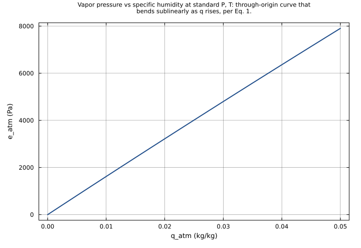
Equation 1 (vapor pressure, Oleson Ch. 1 p.17): e_atm = q_atm * P_atm / (epsilon + (1-epsilon) * q_atm), where epsilon = MW_wv/MW_da. The Bolton-style mixing-ratio-to-vapor-pressure inversion. Singularities are non-physical: the denominator is bounded below by min(epsilon, 1-epsilon) = 0.378 for q_atm in [0,1], so the division is always well defined. At q_atm = 0, e_atm = 0 (dry air); as q_atm grows, e_atm approaches the asymptote q_atm * P_atm / (1-epsilon).
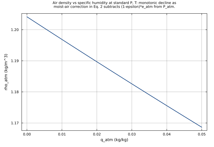
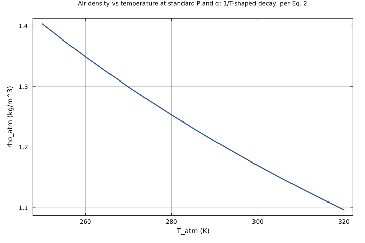
Equation 2 (air density, Oleson Ch. 1 p.17): rho_atm = (P_atm - (1-epsilon) * e_atm) / (R_da * T_atm) — ideal-gas equation of state with humidity correction. Coupled to Eq. 1 via e_atm; the runner resolves them in the order Eq.1 → Eq.2.
Equation 3 (reference height, Oleson Ch. 1 Footnote 1 p.16): z_atm = z_prime_atm + z_0 + z_d. The atmospheric model reports its reference height z’_atm above some local zero datum; the urban canopy uses an effective z_atm that includes the displacement height z_d (the height above which the log-law wind profile applies) and the roughness length z_0. Pure linear sum; no coupling to the thermodynamic state.
Observability classification: this component is functionally observed-only — the three state variables are each given by a single algebraic equation in terms of parameters (the (t) time index on the upstream @variables has no role since there are no derivatives). Test scenarios use time_span: [0, 1] and sample at t=0 to mirror the convention used by sibling observed-only ESM files in this rig (surface_energy_flux.esm, heating_cooling_flux.esm, phase_change_energy.esm).
Tolerance rationale (model-level rel=1.0e-10): three observed-only algebraic equations (no ODE integration). Eq. 1 is one multiplication, one addition in the denominator, one division; Eq. 2 is one multiplication, one subtraction, one multiplication, one division; Eq. 3 is two additions. All operations are at IEEE-754 ULP precision (~1e-16). The upstream Equation Verification - Vapor Pressure and Equation Verification - Reference Height tests use rtol = 1.0e-10, matched here; Equation Verification - Air Density uses rtol = 1.0e-6 because the upstream test rounded R_da to 287.042 in its analytical reference but lets the actual computed R_da (with full precision) drive the test — here the precomputed R_da default carries the full Julia-precision value, so the test compares full-precision to full-precision and we re-assert at rtol = 1.0e-10. Tighter abs: 1e-12 is asserted on outputs that are exactly zero by construction (e.g. q_atm = 0 → e_atm = 0) so the assertion does not silently accept a stuck-at-zero regression._
Parameters
| Name | Units | Default | Description |
|---|---|---|---|
kappa_boltz | J/K | 1.38065e-23 | Boltzmann constant (Oleson Table 1.4) — upstream @constants κ_boltz; the per-particle gas constant for Avogadro-scaling the universal gas constant |
N_A | mol^-1 | 6.02214e+23 | Avogadro’s number (Oleson Table 1.4) — upstream @constants N_A; the conversion factor from per-mole to per-particle (Oleson uses kmol in the table; this value is converted to SI mol) |
MW_da | kg/mol | 0.028966 | Molecular weight of dry air (Oleson Table 1.4) — upstream @constants MW_da; standard atmospheric mean (Oleson reports 28.966 kg/kmol; here in SI kg/mol) |
MW_wv | kg/mol | 0.018016 | Molecular weight of water vapor (Oleson Table 1.4) — upstream @constants MW_wv; standard H2O molecular weight (Oleson reports 18.016 kg/kmol; here in SI kg/mol) |
R_gas | J/(K*mol) | 8.314467591 | Universal gas constant R_gas = N_A * kappa_boltz (Oleson Table 1.4) — upstream @constants R_gas; the IEEE-754 double-precision product of the upstream Avogadro and Boltzmann defaults (matches Julia bit-for-bit). Not used in this component’s equations but preserved as part of the upstream component’s public constant interface |
R_da | J/(K*kg) | 287.0423113650487 | Specific gas constant for dry air R_da = R_gas / MW_da (Oleson Table 1.4) — upstream @constants R_da; appears as the denominator scale of the ideal-gas law in Eq. 2 of this component. The IEEE-754 double-precision quotient of the upstream R_gas / MW_da defaults (matches Julia bit-for-bit, slightly tighter than the rounded 287.042 used in the upstream test docstring) |
epsilon_ratio | 1 | 0.6219705862045157 | Ratio of molecular weights epsilon = MW_wv / MW_da (Oleson Table 1.4) — upstream @constants ε_ratio; appears in the denominator of the vapor-pressure inversion (Eq. 1). The IEEE-754 double-precision quotient of MW_wv / MW_da (matches Julia bit-for-bit; commonly rounded to 0.622 in textbook references) |
one_minus_epsilon | 1 | 0.37802941379548427 | Complement 1 - epsilon = 1 - MW_wv / MW_da (Oleson Table 1.4) — upstream @constants one_minus_ε; appears as the coefficient of q_atm in the vapor-pressure denominator (Eq. 1) and as the coefficient of e_atm in the air-density numerator (Eq. 2). The IEEE-754 double-precision 1.0 - epsilon_ratio (commonly rounded to 0.378) |
z_prime_atm | m | 30.0 | Atmospheric reference height from the driving atmospheric model (Oleson Table 1.1) — z’_atm, the height above the zero datum at which the atmospheric forcing variables are reported. Combined with z_0 and z_d in Eq. 3 to produce the effective z_atm used by the urban-canopy flux computations |
u_atm | m/s | 0.0 | Zonal wind at the atmospheric reference height (Oleson Table 1.1) — passthrough atmospheric forcing input consumed by downstream urban-canopy momentum-flux components; declared by the upstream interface component but not used in the three diagnostic equations of CLMUAtmosphere itself |
v_atm | m/s | 0.0 | Meridional wind at the atmospheric reference height (Oleson Table 1.1) — passthrough atmospheric forcing input consumed by downstream urban-canopy momentum-flux components; declared by the upstream interface component but not used in the three diagnostic equations of CLMUAtmosphere itself |
theta_atm | K | 293.15 | Atmospheric potential temperature at the reference height (Oleson Table 1.1) — upstream @parameters θ_atm; passthrough atmospheric forcing input consumed by downstream urban-canopy sensible-heat-flux components; declared by the upstream interface component but not used in the three diagnostic equations of CLMUAtmosphere itself |
q_atm | kg/kg | 0.01 | Specific humidity at the atmospheric reference height (Oleson Table 1.1) — input to the vapor-pressure inversion (Eq. 1) and indirectly the air-density correction (Eq. 2). Mass of water vapor per mass of moist air; typical mid-latitude values 0.001-0.02 kg/kg |
P_atm | Pa | 101325.0 | Atmospheric pressure at the reference height (Oleson Table 1.1) — total pressure, input to both Eq. 1 (numerator of vapor-pressure inversion) and Eq. 2 (numerator of ideal-gas law). Default is the standard sea-level atmosphere (101325 Pa) |
T_atm | K | 293.15 | Atmospheric temperature at the reference height (Oleson Table 1.1) — input to the ideal-gas air-density equation (Eq. 2). Default is the standard sea-level temperature (293.15 K = 20 degC) |
L_atm_down | W/m^2 | 0.0 | Incident downward longwave radiation at the reference height (Oleson Table 1.1) — passthrough atmospheric forcing input consumed by downstream urban-canopy longwave-flux components; declared by the upstream interface component but not used in the three diagnostic equations of CLMUAtmosphere itself |
q_rain | kg/(m^2*s) | 0.0 | Liquid precipitation rate (Oleson Table 1.1) — passthrough atmospheric forcing input consumed by downstream urban-canopy hydrology components; declared by the upstream interface component but not used in the three diagnostic equations of CLMUAtmosphere itself |
q_sno | kg/(m^2*s) | 0.0 | Solid precipitation rate (Oleson Table 1.1) — passthrough atmospheric forcing input consumed by downstream urban-canopy snow components; declared by the upstream interface component but not used in the three diagnostic equations of CLMUAtmosphere itself |
S_atm_dir_vis | W/m^2 | 0.0 | Incident direct-beam visible solar radiation (Oleson Table 1.1) — passthrough atmospheric forcing input consumed by downstream urban-canopy shortwave-radiation components; declared by the upstream interface component but not used in the three diagnostic equations of CLMUAtmosphere itself |
S_atm_dir_nir | W/m^2 | 0.0 | Incident direct-beam near-infrared solar radiation (Oleson Table 1.1) — passthrough atmospheric forcing input consumed by downstream urban-canopy shortwave-radiation components; declared by the upstream interface component but not used in the three diagnostic equations of CLMUAtmosphere itself |
S_atm_dif_vis | W/m^2 | 0.0 | Incident diffuse visible solar radiation (Oleson Table 1.1) — passthrough atmospheric forcing input consumed by downstream urban-canopy shortwave-radiation components; declared by the upstream interface component but not used in the three diagnostic equations of CLMUAtmosphere itself |
S_atm_dif_nir | W/m^2 | 0.0 | Incident diffuse near-infrared solar radiation (Oleson Table 1.1) — passthrough atmospheric forcing input consumed by downstream urban-canopy shortwave-radiation components; declared by the upstream interface component but not used in the three diagnostic equations of CLMUAtmosphere itself |
z_0 | m | 1.0 | Roughness length (Oleson Table 1.3, Footnote 1 p.16) — characteristic length scale of the surface drag for the log-law wind profile. Typical urban values 0.5-3 m. Input to Eq. 3 (effective reference height) |
z_d | m | 5.0 | Displacement height (Oleson Table 1.3, Footnote 1 p.16) — vertical offset of the log-law wind profile, representing the effective height of the canopy bulk drag center. Typical urban values 1-15 m (a fraction of building height H). Input to Eq. 3 (effective reference height) |
Observed
| Name | Units | Default | Description |
|---|---|---|---|
e_atm | Pa | Atmospheric vapor pressure (Oleson Ch. 1 p.17, Eq. 1): e_atm = q_atm * P_atm / (epsilon + (1-epsilon) * q_atm). Bolton-style inversion of specific humidity to vapor pressure for the moist-air state used by downstream flux components. At q_atm = 0 gives e_atm = 0; bounded above by P_atm at q_atm = 1 | |
rho_atm | kg/m^3 | Atmospheric air density (Oleson Ch. 1 p.17, Eq. 2): rho_atm = (P_atm - (1-epsilon) * e_atm) / (R_da * T_atm). Ideal-gas density of moist air, with the (1-epsilon)e_atm correction subtracted from P_atm to give the dry-air partial pressure (which then divides by R_daT_atm). The humidity correction makes moist air slightly less dense than dry air at the same P and T | |
z_atm | m | Effective atmospheric reference height for flux computations (Oleson Ch. 1 Footnote 1 p.16, Eq. 3): z_atm = z_prime_atm + z_0 + z_d. Linear sum of the model-reported height and the surface drag-profile parameters; used by downstream urban-canopy momentum and turbulent-flux subcomponents as the height at which the atmospheric forcings are evaluated |
Observed expressions
$$ e_{atm} = \frac{q_{atm} \cdot P_{atm}}{epsilon_{ratio} + one_{minus\,epsilon} \cdot q_{atm}} $$Atmospheric vapor pressure (Oleson Ch. 1 p.17, Eq. 1): e_atm = q_atm * P_atm / (epsilon + (1-epsilon) * q_atm). Bolton-style inversion of specific humidity to vapor pressure for the moist-air state used by downstream flux components. At q_atm = 0 gives e_atm = 0; bounded above by P_atm at q_atm = 1
$$ rho_{atm} = \frac{P_{atm} - one_{minus\,epsilon} \cdot e_{atm}}{R_{da} \cdot T_{atm}} $$Atmospheric air density (Oleson Ch. 1 p.17, Eq. 2): rho_atm = (P_atm - (1-epsilon) * e_atm) / (R_da * T_atm). Ideal-gas density of moist air, with the (1-epsilon)e_atm correction subtracted from P_atm to give the dry-air partial pressure (which then divides by R_daT_atm). The humidity correction makes moist air slightly less dense than dry air at the same P and T
$$ z_{atm} = z_{prime\,atm} + z_{0} + z_{d} $$Effective atmospheric reference height for flux computations (Oleson Ch. 1 Footnote 1 p.16, Eq. 3): z_atm = z_prime_atm + z_0 + z_d. Linear sum of the model-reported height and the surface drag-profile parameters; used by downstream urban-canopy momentum and turbulent-flux subcomponents as the height at which the atmospheric forcings are evaluated
Analyses
vapor_pressure_vs_specific_humidity_sweep
Sweep q_atm from 0 to 0.05 kg/kg at fixed P_atm = 101325 Pa, T_atm = 293.15 K to surface the vapor-pressure inversion (Eq. 1): e_atm = q_atm * P_atm / (epsilon + (1-epsilon) * q_atm). The curve passes through the origin (q = 0 → e = 0) and grows nearly linearly at small q with slope P_atm / epsilon ≈ 162900 Pa per (kg/kg), bending sublinearly as the denominator (1-epsilon)*q_atm starts to compete with epsilon. The accompanying rho_atm curve drops as q_atm rises, mirroring the (1-epsilon)*e_atm humidity correction in Eq. 2.
Time span: 0.0 → 1.0
Swept over: q_atm
air_density_temperature_sweep
Sweep T_atm from 250 to 320 K at fixed P_atm = 101325 Pa, q_atm = 0.01 kg/kg, surfacing the 1/T scaling of the ideal-gas law (Eq. 2). e_atm is T-independent (Eq. 1 has no T term) so it stays flat at 1619.25 Pa across the sweep; rho_atm drops smoothly from 1.412 kg/m^3 at 250 K to 1.097 kg/m^3 at 320 K, exhibiting the strong negative dependence on temperature that drives buoyancy in convective boundary layers.
Time span: 0.0 → 1.0
Swept over: T_atm
air_density_pressure_temperature_heatmap
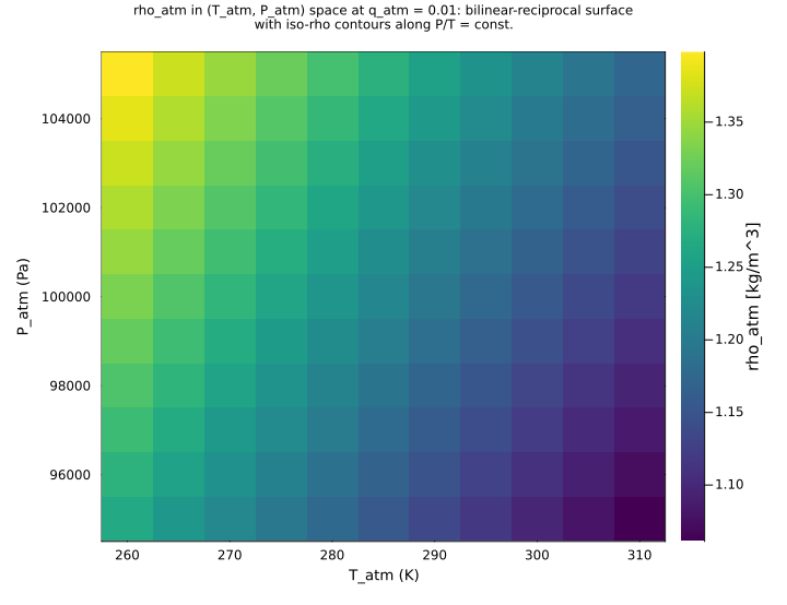
Joint sweep over (T_atm, P_atm) at fixed q_atm = 0.01 kg/kg, showing the bilinear-reciprocal structure of Eq. 2: rho_atm grows linearly with P_atm at fixed T and decays as 1/T at fixed P. Iso-rho contours follow curves of constant P/T (isentropes for an ideal gas), useful for visualizing the parameter regime of typical urban boundary-layer states (P in [95, 105] kPa, T in [260, 310] K spanning winter to summer).
Time span: 0.0 → 1.0
Swept over: T_atm, P_atm
Raw .esm
Raw .esm JSON (this component)
{
"reference": {
"notes": "source_ref: UrbanCanopy.jl@9200edd4f15609f20339d3a7d104de8064544310:src/clmu_introduction.jl:22\nUpstream `CLMUAtmosphere` is an MTK `@component` with two `@constants` blocks (4 base constants + 4 derived constants), two `@parameters` blocks (14 atmospheric forcing inputs + 2 surface parameters), three time-indexed `@variables` (e_atm, rho_atm, z_atm), and three algebraic equations (no derivatives). Identical equation structure preserved here.\n\nConstants encoding (mirrors surface_energy_flux.esm/heat_flux.esm/heating_cooling_flux.esm sibling pattern of encoding upstream `@constants` as fixed-default parameters so the units flow through the unit checker): the four base constants from Oleson Table 1.4 (kappa_boltz = 1.38065e-23 J/K Boltzmann, N_A = 6.02214e23 /mol Avogadro, MW_da = 0.028966 kg/mol dry-air molecular weight, MW_wv = 0.018016 kg/mol water-vapor molecular weight) are encoded with their upstream defaults; the four derived constants (R_gas = N_A * kappa_boltz = 8.314467591 J/(K*mol) universal gas constant, R_da = R_gas / MW_da = 287.0423113650487 J/(K*kg) dry-air specific gas constant, epsilon_ratio = MW_wv/MW_da = 0.6219705862045157 dimensionless, one_minus_epsilon = 1 - MW_wv/MW_da = 0.37802941379548427 dimensionless) are encoded with their IEEE-754-double-precision pre-computed values from those bases. The pre-computed values are exactly what Julia computes for the same `@constants` expressions at MTK macro-expansion time, so the diagnostic outputs match the upstream test fixtures bit-for-bit (e.g. e_atm at q=0.01, P=101325 is 1619.2546136658295 Pa in both this ESM and the upstream test).\n\nGreek-to-ASCII identifier renaming (rig convention, matches surface_energy_flux.esm σ_SB → sigma_SB / ε_g → epsilon_g / λE_g → lambdaE_g, and snow_density.esm rho_*): upstream `κ_boltz` → `kappa_boltz`, `ε_ratio` → `epsilon_ratio`, `one_minus_ε` → `one_minus_epsilon`, `θ_atm` → `theta_atm`, `ρ_atm` → `rho_atm`. ASCII identifiers (`N_A`, `MW_da`, `MW_wv`, `R_gas`, `R_da`, `e_atm`, `z_atm`, `q_atm`, `P_atm`, `T_atm`, `z_prime_atm`, `u_atm`, `v_atm`, `q_rain`, `q_sno`, `L_atm_down`, `S_atm_*`, `z_0`, `z_d`) are preserved verbatim.\n\nAtmospheric-forcing parameters preserved: the upstream component declares 14 forcing parameters from Oleson Table 1.1 (wind components u_atm/v_atm, potential temperature theta_atm, specific humidity q_atm, pressure P_atm, temperature T_atm, downward longwave L_atm_down, precip q_rain/q_sno, direct/diffuse vis/nir solar fluxes S_atm_dir_vis/S_atm_dir_nir/S_atm_dif_vis/S_atm_dif_nir, and the model-provided reference height z_prime_atm) plus 2 surface parameters from Table 1.3 Footnote 1 (z_0 roughness length, z_d displacement height). Only q_atm, P_atm, T_atm, z_prime_atm, z_0, z_d, epsilon_ratio, one_minus_epsilon, R_da appear in the 3 diagnostic equations; the remaining forcing inputs (u_atm, v_atm, theta_atm, L_atm_down, q_rain, q_sno, S_atm_*) are interface passthroughs that downstream urban-canopy components consume via the upstream coupling.couple mechanism — they are preserved as parameters here to match the upstream component's external interface contract (the upstream `Structural Verification` test verifies the parameter set via `parameters(sys)`).\n\nEquation 1 (vapor pressure, Oleson Ch. 1 p.17): e_atm = q_atm * P_atm / (epsilon + (1-epsilon) * q_atm), where epsilon = MW_wv/MW_da. The Bolton-style mixing-ratio-to-vapor-pressure inversion. Singularities are non-physical: the denominator is bounded below by min(epsilon, 1-epsilon) = 0.378 for q_atm in [0,1], so the division is always well defined. At q_atm = 0, e_atm = 0 (dry air); as q_atm grows, e_atm approaches the asymptote q_atm * P_atm / (1-epsilon).\n\nEquation 2 (air density, Oleson Ch. 1 p.17): rho_atm = (P_atm - (1-epsilon) * e_atm) / (R_da * T_atm) — ideal-gas equation of state with humidity correction. Coupled to Eq. 1 via e_atm; the runner resolves them in the order Eq.1 → Eq.2.\n\nEquation 3 (reference height, Oleson Ch. 1 Footnote 1 p.16): z_atm = z_prime_atm + z_0 + z_d. The atmospheric model reports its reference height z'_atm above some local zero datum; the urban canopy uses an effective z_atm that includes the displacement height z_d (the height above which the log-law wind profile applies) and the roughness length z_0. Pure linear sum; no coupling to the thermodynamic state.\n\nObservability classification: this component is functionally observed-only — the three state variables are each given by a single algebraic equation in terms of parameters (the `(t)` time index on the upstream `@variables` has no role since there are no derivatives). Test scenarios use `time_span: [0, 1]` and sample at t=0 to mirror the convention used by sibling observed-only ESM files in this rig (surface_energy_flux.esm, heating_cooling_flux.esm, phase_change_energy.esm).\n\nTolerance rationale (model-level rel=1.0e-10): three observed-only algebraic equations (no ODE integration). Eq. 1 is one multiplication, one addition in the denominator, one division; Eq. 2 is one multiplication, one subtraction, one multiplication, one division; Eq. 3 is two additions. All operations are at IEEE-754 ULP precision (~1e-16). The upstream `Equation Verification - Vapor Pressure` and `Equation Verification - Reference Height` tests use `rtol = 1.0e-10`, matched here; `Equation Verification - Air Density` uses `rtol = 1.0e-6` because the upstream test rounded R_da to 287.042 in its analytical reference but lets the actual computed R_da (with full precision) drive the test — here the precomputed R_da default carries the full Julia-precision value, so the test compares full-precision to full-precision and we re-assert at rtol = 1.0e-10. Tighter `abs: 1e-12` is asserted on outputs that are exactly zero by construction (e.g. q_atm = 0 → e_atm = 0) so the assertion does not silently accept a stuck-at-zero regression."
},
"tolerance": {
"rel": 1e-10
},
"variables": {
"kappa_boltz": {
"type": "parameter",
"units": "J/K",
"default": 1.38065e-23,
"description": "Boltzmann constant (Oleson Table 1.4) — upstream `@constants` κ_boltz; the per-particle gas constant for Avogadro-scaling the universal gas constant"
},
"N_A": {
"type": "parameter",
"units": "mol^-1",
"default": 6.02214e+23,
"description": "Avogadro's number (Oleson Table 1.4) — upstream `@constants` N_A; the conversion factor from per-mole to per-particle (Oleson uses kmol in the table; this value is converted to SI mol)"
},
"MW_da": {
"type": "parameter",
"units": "kg/mol",
"default": 0.028966,
"description": "Molecular weight of dry air (Oleson Table 1.4) — upstream `@constants` MW_da; standard atmospheric mean (Oleson reports 28.966 kg/kmol; here in SI kg/mol)"
},
"MW_wv": {
"type": "parameter",
"units": "kg/mol",
"default": 0.018016,
"description": "Molecular weight of water vapor (Oleson Table 1.4) — upstream `@constants` MW_wv; standard H2O molecular weight (Oleson reports 18.016 kg/kmol; here in SI kg/mol)"
},
"R_gas": {
"type": "parameter",
"units": "J/(K*mol)",
"default": 8.314467591,
"description": "Universal gas constant R_gas = N_A * kappa_boltz (Oleson Table 1.4) — upstream `@constants` R_gas; the IEEE-754 double-precision product of the upstream Avogadro and Boltzmann defaults (matches Julia bit-for-bit). Not used in this component's equations but preserved as part of the upstream component's public constant interface"
},
"R_da": {
"type": "parameter",
"units": "J/(K*kg)",
"default": 287.0423113650487,
"description": "Specific gas constant for dry air R_da = R_gas / MW_da (Oleson Table 1.4) — upstream `@constants` R_da; appears as the denominator scale of the ideal-gas law in Eq. 2 of this component. The IEEE-754 double-precision quotient of the upstream R_gas / MW_da defaults (matches Julia bit-for-bit, slightly tighter than the rounded 287.042 used in the upstream test docstring)"
},
"epsilon_ratio": {
"type": "parameter",
"units": "1",
"default": 0.6219705862045157,
"description": "Ratio of molecular weights epsilon = MW_wv / MW_da (Oleson Table 1.4) — upstream `@constants` ε_ratio; appears in the denominator of the vapor-pressure inversion (Eq. 1). The IEEE-754 double-precision quotient of MW_wv / MW_da (matches Julia bit-for-bit; commonly rounded to 0.622 in textbook references)"
},
"one_minus_epsilon": {
"type": "parameter",
"units": "1",
"default": 0.37802941379548427,
"description": "Complement 1 - epsilon = 1 - MW_wv / MW_da (Oleson Table 1.4) — upstream `@constants` one_minus_ε; appears as the coefficient of q_atm in the vapor-pressure denominator (Eq. 1) and as the coefficient of e_atm in the air-density numerator (Eq. 2). The IEEE-754 double-precision 1.0 - epsilon_ratio (commonly rounded to 0.378)"
},
"z_prime_atm": {
"type": "parameter",
"units": "m",
"default": 30.0,
"description": "Atmospheric reference height from the driving atmospheric model (Oleson Table 1.1) — z'_atm, the height above the zero datum at which the atmospheric forcing variables are reported. Combined with z_0 and z_d in Eq. 3 to produce the effective z_atm used by the urban-canopy flux computations"
},
"u_atm": {
"type": "parameter",
"units": "m/s",
"default": 0.0,
"description": "Zonal wind at the atmospheric reference height (Oleson Table 1.1) — passthrough atmospheric forcing input consumed by downstream urban-canopy momentum-flux components; declared by the upstream interface component but not used in the three diagnostic equations of CLMUAtmosphere itself"
},
"v_atm": {
"type": "parameter",
"units": "m/s",
"default": 0.0,
"description": "Meridional wind at the atmospheric reference height (Oleson Table 1.1) — passthrough atmospheric forcing input consumed by downstream urban-canopy momentum-flux components; declared by the upstream interface component but not used in the three diagnostic equations of CLMUAtmosphere itself"
},
"theta_atm": {
"type": "parameter",
"units": "K",
"default": 293.15,
"description": "Atmospheric potential temperature at the reference height (Oleson Table 1.1) — upstream `@parameters` θ_atm; passthrough atmospheric forcing input consumed by downstream urban-canopy sensible-heat-flux components; declared by the upstream interface component but not used in the three diagnostic equations of CLMUAtmosphere itself"
},
"q_atm": {
"type": "parameter",
"units": "kg/kg",
"default": 0.01,
"description": "Specific humidity at the atmospheric reference height (Oleson Table 1.1) — input to the vapor-pressure inversion (Eq. 1) and indirectly the air-density correction (Eq. 2). Mass of water vapor per mass of moist air; typical mid-latitude values 0.001-0.02 kg/kg"
},
"P_atm": {
"type": "parameter",
"units": "Pa",
"default": 101325.0,
"description": "Atmospheric pressure at the reference height (Oleson Table 1.1) — total pressure, input to both Eq. 1 (numerator of vapor-pressure inversion) and Eq. 2 (numerator of ideal-gas law). Default is the standard sea-level atmosphere (101325 Pa)"
},
"T_atm": {
"type": "parameter",
"units": "K",
"default": 293.15,
"description": "Atmospheric temperature at the reference height (Oleson Table 1.1) — input to the ideal-gas air-density equation (Eq. 2). Default is the standard sea-level temperature (293.15 K = 20 degC)"
},
"L_atm_down": {
"type": "parameter",
"units": "W/m^2",
"default": 0.0,
"description": "Incident downward longwave radiation at the reference height (Oleson Table 1.1) — passthrough atmospheric forcing input consumed by downstream urban-canopy longwave-flux components; declared by the upstream interface component but not used in the three diagnostic equations of CLMUAtmosphere itself"
},
"q_rain": {
"type": "parameter",
"units": "kg/(m^2*s)",
"default": 0.0,
"description": "Liquid precipitation rate (Oleson Table 1.1) — passthrough atmospheric forcing input consumed by downstream urban-canopy hydrology components; declared by the upstream interface component but not used in the three diagnostic equations of CLMUAtmosphere itself"
},
"q_sno": {
"type": "parameter",
"units": "kg/(m^2*s)",
"default": 0.0,
"description": "Solid precipitation rate (Oleson Table 1.1) — passthrough atmospheric forcing input consumed by downstream urban-canopy snow components; declared by the upstream interface component but not used in the three diagnostic equations of CLMUAtmosphere itself"
},
"S_atm_dir_vis": {
"type": "parameter",
"units": "W/m^2",
"default": 0.0,
"description": "Incident direct-beam visible solar radiation (Oleson Table 1.1) — passthrough atmospheric forcing input consumed by downstream urban-canopy shortwave-radiation components; declared by the upstream interface component but not used in the three diagnostic equations of CLMUAtmosphere itself"
},
"S_atm_dir_nir": {
"type": "parameter",
"units": "W/m^2",
"default": 0.0,
"description": "Incident direct-beam near-infrared solar radiation (Oleson Table 1.1) — passthrough atmospheric forcing input consumed by downstream urban-canopy shortwave-radiation components; declared by the upstream interface component but not used in the three diagnostic equations of CLMUAtmosphere itself"
},
"S_atm_dif_vis": {
"type": "parameter",
"units": "W/m^2",
"default": 0.0,
"description": "Incident diffuse visible solar radiation (Oleson Table 1.1) — passthrough atmospheric forcing input consumed by downstream urban-canopy shortwave-radiation components; declared by the upstream interface component but not used in the three diagnostic equations of CLMUAtmosphere itself"
},
"S_atm_dif_nir": {
"type": "parameter",
"units": "W/m^2",
"default": 0.0,
"description": "Incident diffuse near-infrared solar radiation (Oleson Table 1.1) — passthrough atmospheric forcing input consumed by downstream urban-canopy shortwave-radiation components; declared by the upstream interface component but not used in the three diagnostic equations of CLMUAtmosphere itself"
},
"z_0": {
"type": "parameter",
"units": "m",
"default": 1.0,
"description": "Roughness length (Oleson Table 1.3, Footnote 1 p.16) — characteristic length scale of the surface drag for the log-law wind profile. Typical urban values 0.5-3 m. Input to Eq. 3 (effective reference height)"
},
"z_d": {
"type": "parameter",
"units": "m",
"default": 5.0,
"description": "Displacement height (Oleson Table 1.3, Footnote 1 p.16) — vertical offset of the log-law wind profile, representing the effective height of the canopy bulk drag center. Typical urban values 1-15 m (a fraction of building height H). Input to Eq. 3 (effective reference height)"
},
"e_atm": {
"type": "unknown",
"units": "Pa",
"description": "Atmospheric vapor pressure (Oleson Ch. 1 p.17, Eq. 1): e_atm = q_atm * P_atm / (epsilon + (1-epsilon) * q_atm). Bolton-style inversion of specific humidity to vapor pressure for the moist-air state used by downstream flux components. At q_atm = 0 gives e_atm = 0; bounded above by P_atm at q_atm = 1"
},
"rho_atm": {
"type": "unknown",
"units": "kg/m^3",
"description": "Atmospheric air density (Oleson Ch. 1 p.17, Eq. 2): rho_atm = (P_atm - (1-epsilon) * e_atm) / (R_da * T_atm). Ideal-gas density of moist air, with the (1-epsilon)*e_atm correction subtracted from P_atm to give the dry-air partial pressure (which then divides by R_da*T_atm). The humidity correction makes moist air slightly less dense than dry air at the same P and T"
},
"z_atm": {
"type": "unknown",
"units": "m",
"description": "Effective atmospheric reference height for flux computations (Oleson Ch. 1 Footnote 1 p.16, Eq. 3): z_atm = z_prime_atm + z_0 + z_d. Linear sum of the model-reported height and the surface drag-profile parameters; used by downstream urban-canopy momentum and turbulent-flux subcomponents as the height at which the atmospheric forcings are evaluated"
}
},
"equations": [
{
"lhs": "e_atm",
"rhs": {
"op": "/",
"args": [
{
"op": "*",
"args": [
"q_atm",
"P_atm"
]
},
{
"op": "+",
"args": [
"epsilon_ratio",
{
"op": "*",
"args": [
"one_minus_epsilon",
"q_atm"
]
}
]
}
]
}
},
{
"lhs": "rho_atm",
"rhs": {
"op": "/",
"args": [
{
"op": "-",
"args": [
"P_atm",
{
"op": "*",
"args": [
"one_minus_epsilon",
"e_atm"
]
}
]
},
{
"op": "*",
"args": [
"R_da",
"T_atm"
]
}
]
}
},
{
"lhs": "z_atm",
"rhs": {
"op": "+",
"args": [
{
"op": "+",
"args": [
"z_prime_atm",
"z_0"
]
},
"z_d"
]
}
}
],
"tests": [
{
"id": "upstream_vapor_pressure_canonical",
"description": "Reproduces upstream `Equation Verification - Vapor Pressure` test (UrbanCanopy.jl test/clmu_introduction_test.jl:71-99) at q_atm = 0.01 kg/kg, P_atm = 101325 Pa, T_atm = 293.15 K. Expected e_atm = 0.01 * 101325 / (0.6219705862 + 0.3780294138 * 0.01) = 1619.2546136658295 Pa (the upstream pre-computed reference). Anchors fidelity to the upstream Julia component at the same parameter values with rtol = 1.0e-10.",
"parameter_overrides": {
"q_atm": 0.01,
"P_atm": 101325.0,
"T_atm": 293.15,
"z_prime_atm": 30.0,
"z_0": 1.0,
"z_d": 5.0
},
"time_span": {
"start": 0.0,
"end": 1.0
},
"assertions": [
{
"variable": "e_atm",
"time": 0.0,
"expected": 1619.2546136658295,
"tolerance": {
"rel": 1e-10
}
}
]
},
{
"id": "upstream_vapor_pressure_dry_air",
"description": "Upstream secondary check from the same test (UrbanCanopy.jl test/clmu_introduction_test.jl:96-98): q_atm = 0 (perfectly dry air) gives e_atm = 0 exactly. The vapor-pressure numerator q_atm * P_atm vanishes; the denominator collapses to epsilon_ratio (non-zero) so the division is well defined. abs tolerance gates the stuck-at-zero failure mode and matches the upstream `atol = 1.0e-15` precision.",
"parameter_overrides": {
"q_atm": 0.0,
"P_atm": 101325.0,
"T_atm": 293.15,
"z_prime_atm": 30.0,
"z_0": 1.0,
"z_d": 5.0
},
"time_span": {
"start": 0.0,
"end": 1.0
},
"assertions": [
{
"variable": "e_atm",
"time": 0.0,
"expected": 0.0,
"tolerance": {
"abs": 1e-15
}
}
]
},
{
"id": "upstream_air_density_dry",
"description": "Reproduces upstream `Equation Verification - Air Density` test for dry air (UrbanCanopy.jl test/clmu_introduction_test.jl:101-123). At q_atm = 0, e_atm = 0 (from Eq. 1) so rho_atm = P_atm / (R_da * T_atm) = 101325 / (287.0423113650487 * 293.15) = 1.2041505695505632 kg/m^3 (the upstream pre-computed reference). Sister assertion confirms e_atm = 0 at the same point so the chain Eq.1 → Eq.2 is independently anchored.",
"parameter_overrides": {
"q_atm": 0.0,
"P_atm": 101325.0,
"T_atm": 293.15,
"z_prime_atm": 30.0,
"z_0": 1.0,
"z_d": 5.0
},
"time_span": {
"start": 0.0,
"end": 1.0
},
"assertions": [
{
"variable": "e_atm",
"time": 0.0,
"expected": 0.0,
"tolerance": {
"abs": 1e-15
}
},
{
"variable": "rho_atm",
"time": 0.0,
"expected": 1.2041505695505632,
"tolerance": {
"rel": 1e-10
}
}
]
},
{
"id": "upstream_air_density_moist",
"description": "Reproduces upstream `Equation Verification - Air Density` test for moist air (UrbanCanopy.jl test/clmu_introduction_test.jl:125-131): rho_atm = (101325 - 0.378 * 1619.25) / (287.042 * 293.15) = 1.1968760398898206 kg/m^3 (the upstream pre-computed reference at q_atm = 0.01). Anchors the (1-epsilon) * e_atm humidity-correction term in Eq. 2: moist air must be slightly less dense than dry air at the same P and T (1.1969 < 1.2042). This is the canonical 'moist air is less dense' check.",
"parameter_overrides": {
"q_atm": 0.01,
"P_atm": 101325.0,
"T_atm": 293.15,
"z_prime_atm": 30.0,
"z_0": 1.0,
"z_d": 5.0
},
"time_span": {
"start": 0.0,
"end": 1.0
},
"assertions": [
{
"variable": "e_atm",
"time": 0.0,
"expected": 1619.2546136658295,
"tolerance": {
"rel": 1e-10
}
},
{
"variable": "rho_atm",
"time": 0.0,
"expected": 1.1968760398898206,
"tolerance": {
"rel": 1e-10
}
}
]
},
{
"id": "upstream_reference_height",
"description": "Reproduces upstream `Equation Verification - Reference Height` test (UrbanCanopy.jl test/clmu_introduction_test.jl:137-160) at z_prime_atm = 30 m, z_0 = 1 m, z_d = 5 m. Expected z_atm = 30 + 1 + 5 = 36 m exactly. Linear-sum identity (Eq. 3); no coupling to thermodynamic state.",
"parameter_overrides": {
"q_atm": 0.01,
"P_atm": 101325.0,
"T_atm": 293.15,
"z_prime_atm": 30.0,
"z_0": 1.0,
"z_d": 5.0
},
"time_span": {
"start": 0.0,
"end": 1.0
},
"assertions": [
{
"variable": "z_atm",
"time": 0.0,
"expected": 36.0,
"tolerance": {
"rel": 1e-10
}
}
]
},
{
"id": "qualitative_high_pressure_higher_density",
"description": "Reproduces upstream `Qualitative Properties` check (test/clmu_introduction_test.jl:184-186): higher P_atm at same T_atm gives higher rho_atm (ideal-gas law monotonicity). At P_atm = 110000 Pa, q_atm = 0.01, T_atm = 293.15: e_atm scales linearly with P_atm (Eq. 1 numerator is q*P, denominator is q-only), so e_atm(110000) = 1757.8880582604613 Pa, then rho_atm = (110000 - one_minus_epsilon * e_atm) / (R_da * T_atm) = 1.2993472922564053 kg/m^3. Higher than the q=0.01, P=101325 reference rho = 1.1968760398898206 — the ideal-gas P/T scaling at constant T outweighs the moist-air correction.",
"parameter_overrides": {
"q_atm": 0.01,
"P_atm": 110000.0,
"T_atm": 293.15,
"z_prime_atm": 30.0,
"z_0": 1.0,
"z_d": 5.0
},
"time_span": {
"start": 0.0,
"end": 1.0
},
"assertions": [
{
"variable": "e_atm",
"time": 0.0,
"expected": 1757.8880582604613,
"tolerance": {
"rel": 1e-10
}
},
{
"variable": "rho_atm",
"time": 0.0,
"expected": 1.2993472922564053,
"tolerance": {
"rel": 1e-10
}
}
]
},
{
"id": "qualitative_high_temperature_lower_density",
"description": "Reproduces upstream `Qualitative Properties` check (test/clmu_introduction_test.jl:188-191): higher T_atm at same P_atm gives lower rho_atm. At T_atm = 313.15 K (40 degC), q_atm = 0.01, P_atm = 101325: e_atm is T-independent (Eq. 1 has no T term) so still 1619.2546136658295 Pa; rho_atm = (101325 - one_minus_epsilon * 1619.25) / (R_da * 313.15) = 1.1204349707606607 kg/m^3. Lower than the T = 293.15 reference rho = 1.1968760398898206 — matches the 1/T scaling of the ideal-gas law.",
"parameter_overrides": {
"q_atm": 0.01,
"P_atm": 101325.0,
"T_atm": 313.15,
"z_prime_atm": 30.0,
"z_0": 1.0,
"z_d": 5.0
},
"time_span": {
"start": 0.0,
"end": 1.0
},
"assertions": [
{
"variable": "e_atm",
"time": 0.0,
"expected": 1619.2546136658295,
"tolerance": {
"rel": 1e-10
}
},
{
"variable": "rho_atm",
"time": 0.0,
"expected": 1.1204349707606607,
"tolerance": {
"rel": 1e-10
}
}
]
},
{
"id": "qualitative_high_humidity_higher_vapor_pressure",
"description": "Reproduces upstream `Qualitative Properties` check (test/clmu_introduction_test.jl:193-196): higher q_atm at same P_atm gives higher e_atm. At q_atm = 0.02, P_atm = 101325: e_atm = 0.02 * 101325 / (epsilon_ratio + one_minus_epsilon * 0.02) = 3219.062188099808 Pa. Strictly greater than the q = 0.01 reference e_atm = 1619.2546 Pa. Sublinear in q_atm: doubling q_atm gives slightly less than double e_atm because the denominator (1-epsilon)*q_atm grows alongside the numerator (asymptotically e_atm → q*P/(1-eps) ≈ q*P/0.378 as q→∞).",
"parameter_overrides": {
"q_atm": 0.02,
"P_atm": 101325.0,
"T_atm": 293.15,
"z_prime_atm": 30.0,
"z_0": 1.0,
"z_d": 5.0
},
"time_span": {
"start": 0.0,
"end": 1.0
},
"assertions": [
{
"variable": "e_atm",
"time": 0.0,
"expected": 3219.062188099808,
"tolerance": {
"rel": 1e-10
}
}
]
},
{
"id": "reference_height_zero_offsets",
"description": "Boundary case for Eq. 3: z_0 = z_d = 0 collapses the effective reference height to the raw atmospheric reference: z_atm = z_prime_atm + 0 + 0 = z_prime_atm. Confirms the linear-sum identity has no hidden offsets and pins the z_prime_atm passthrough behavior at the zero-surface limit (smooth bare ground).",
"parameter_overrides": {
"q_atm": 0.0,
"P_atm": 101325.0,
"T_atm": 293.15,
"z_prime_atm": 20.0,
"z_0": 0.0,
"z_d": 0.0
},
"time_span": {
"start": 0.0,
"end": 1.0
},
"assertions": [
{
"variable": "z_atm",
"time": 0.0,
"expected": 20.0,
"tolerance": {
"rel": 1e-10
}
}
]
}
],
"analyses": [
{
"id": "vapor_pressure_vs_specific_humidity_sweep",
"description": "Sweep q_atm from 0 to 0.05 kg/kg at fixed P_atm = 101325 Pa, T_atm = 293.15 K to surface the vapor-pressure inversion (Eq. 1): e_atm = q_atm * P_atm / (epsilon + (1-epsilon) * q_atm). The curve passes through the origin (q = 0 → e = 0) and grows nearly linearly at small q with slope P_atm / epsilon ≈ 162900 Pa per (kg/kg), bending sublinearly as the denominator (1-epsilon)*q_atm starts to compete with epsilon. The accompanying rho_atm curve drops as q_atm rises, mirroring the (1-epsilon)*e_atm humidity correction in Eq. 2.",
"initial_state": {},
"parameters": {
"P_atm": 101325.0,
"T_atm": 293.15,
"z_prime_atm": 30.0,
"z_0": 1.0,
"z_d": 5.0
},
"time_span": {
"start": 0.0,
"end": 1.0
},
"parameter_sweep": {
"type": "cartesian",
"dimensions": [
{
"parameter": "q_atm",
"range": {
"start": 0.0,
"stop": 0.05,
"count": 21,
"scale": "linear"
}
}
]
},
"plots": [
{
"id": "e_atm_vs_q",
"type": "line",
"description": "Vapor pressure vs specific humidity at standard P, T: through-origin curve that bends sublinearly as q rises, per Eq. 1.",
"x": {
"variable": "q_atm",
"label": "q_atm (kg/kg)"
},
"y": {
"variable": "e_atm",
"label": "e_atm (Pa)"
}
},
{
"id": "rho_atm_vs_q",
"type": "line",
"description": "Air density vs specific humidity at standard P, T: monotonic decline as moist-air correction in Eq. 2 subtracts (1-epsilon)*e_atm from P_atm.",
"x": {
"variable": "q_atm",
"label": "q_atm (kg/kg)"
},
"y": {
"variable": "rho_atm",
"label": "rho_atm (kg/m^3)"
}
}
]
},
{
"id": "air_density_temperature_sweep",
"description": "Sweep T_atm from 250 to 320 K at fixed P_atm = 101325 Pa, q_atm = 0.01 kg/kg, surfacing the 1/T scaling of the ideal-gas law (Eq. 2). e_atm is T-independent (Eq. 1 has no T term) so it stays flat at 1619.25 Pa across the sweep; rho_atm drops smoothly from 1.412 kg/m^3 at 250 K to 1.097 kg/m^3 at 320 K, exhibiting the strong negative dependence on temperature that drives buoyancy in convective boundary layers.",
"initial_state": {},
"parameters": {
"q_atm": 0.01,
"P_atm": 101325.0,
"z_prime_atm": 30.0,
"z_0": 1.0,
"z_d": 5.0
},
"time_span": {
"start": 0.0,
"end": 1.0
},
"parameter_sweep": {
"type": "cartesian",
"dimensions": [
{
"parameter": "T_atm",
"range": {
"start": 250.0,
"stop": 320.0,
"count": 15,
"scale": "linear"
}
}
]
},
"plots": [
{
"id": "rho_atm_vs_T",
"type": "line",
"description": "Air density vs temperature at standard P and q: 1/T-shaped decay, per Eq. 2.",
"x": {
"variable": "T_atm",
"label": "T_atm (K)"
},
"y": {
"variable": "rho_atm",
"label": "rho_atm (kg/m^3)"
}
}
]
},
{
"id": "air_density_pressure_temperature_heatmap",
"description": "Joint sweep over (T_atm, P_atm) at fixed q_atm = 0.01 kg/kg, showing the bilinear-reciprocal structure of Eq. 2: rho_atm grows linearly with P_atm at fixed T and decays as 1/T at fixed P. Iso-rho contours follow curves of constant P/T (isentropes for an ideal gas), useful for visualizing the parameter regime of typical urban boundary-layer states (P in [95, 105] kPa, T in [260, 310] K spanning winter to summer).",
"initial_state": {},
"parameters": {
"q_atm": 0.01,
"z_prime_atm": 30.0,
"z_0": 1.0,
"z_d": 5.0
},
"time_span": {
"start": 0.0,
"end": 1.0
},
"parameter_sweep": {
"type": "cartesian",
"dimensions": [
{
"parameter": "T_atm",
"range": {
"start": 260.0,
"stop": 310.0,
"count": 11,
"scale": "linear"
}
},
{
"parameter": "P_atm",
"range": {
"start": 95000.0,
"stop": 105000.0,
"count": 11,
"scale": "linear"
}
}
]
},
"plots": [
{
"id": "rho_atm_T_P_heatmap",
"type": "heatmap",
"description": "rho_atm in (T_atm, P_atm) space at q_atm = 0.01: bilinear-reciprocal surface with iso-rho contours along P/T = const.",
"x": {
"variable": "T_atm",
"label": "T_atm (K)"
},
"y": {
"variable": "P_atm",
"label": "P_atm (Pa)"
},
"value": {
"variable": "rho_atm",
"reduce": "final"
}
}
]
}
]
}