ClimateSensitivity
Climate-sensitivity diagnostic (Seinfeld & Pandis 2006 Ch. 4, Eqs. 4.8-4.10) — the linear-response relation between a top-of-atmosphere radiative-forcing perturbation ΔF_net and the resulting change in planetary equilibrium temperature ΔT_e through the no-feedback climate-sensitivity factor λ_0 = 1 / (4·σ·T_e^3) = T_e / (4·F_L). The component is observed-only: four algebraic equations on four state variables (ΔF_net the net forcing, λ_0 the sensitivity factor, ΔT_e the temperature response, F_L the reference longwave flux) driven by three input parameters (T_e the reference equilibrium temperature, ΔF_S the forcing-side perturbation, ΔF_L the longwave-side perturbation) and one constant (σ the Stefan-Boltzmann constant). No time derivatives, no PDE, no coupling. Migrated from GasChem.jl@8c12c048 src/radiation_fundamentals.jl:268 (`ClimateSensitivity` @component). The blackbody reference state (F_L = σ·T_e^4) and the analytic differentiation of Stefan-Boltzmann (dF_L/dT_e = 4·σ·T_e^3 → λ_0 = 1 / (4·σ·T_e^3)) together encode the no-feedback Planck response — the only baseline against which feedback-amplified climate sensitivities (water vapor, lapse rate, albedo, cloud) are conventionally reported in IPCC assessments. At Earth's nominal T_e = 255 K the component reproduces the textbook λ_0 ≈ 0.27 K·m^2/W and a CO2-doubling ΔT_e ≈ 1.22 K (S&P Page 105) using a forcing-doubling estimate of 4.6 W/m^2.
Description
Climate-sensitivity diagnostic (Seinfeld & Pandis 2006 Ch. 4, Eqs. 4.8-4.10) — the linear-response relation between a top-of-atmosphere radiative-forcing perturbation ΔF_net and the resulting change in planetary equilibrium temperature ΔT_e through the no-feedback climate-sensitivity factor λ_0 = 1 / (4·σ·T_e^3) = T_e / (4·F_L). The component is observed-only: four algebraic equations on four state variables (ΔF_net the net forcing, λ_0 the sensitivity factor, ΔT_e the temperature response, F_L the reference longwave flux) driven by three input parameters (T_e the reference equilibrium temperature, ΔF_S the forcing-side perturbation, ΔF_L the longwave-side perturbation) and one constant (σ the Stefan-Boltzmann constant). No time derivatives, no PDE, no coupling. Migrated from GasChem.jl@8c12c048 src/radiation_fundamentals.jl:268 (ClimateSensitivity @component). The blackbody reference state (F_L = σ·T_e^4) and the analytic differentiation of Stefan-Boltzmann (dF_L/dT_e = 4·σ·T_e^3 → λ_0 = 1 / (4·σ·T_e^3)) together encode the no-feedback Planck response — the only baseline against which feedback-amplified climate sensitivities (water vapor, lapse rate, albedo, cloud) are conventionally reported in IPCC assessments. At Earth’s nominal T_e = 255 K the component reproduces the textbook λ_0 ≈ 0.27 K·m^2/W and a CO2-doubling ΔT_e ≈ 1.22 K (S&P Page 105) using a forcing-doubling estimate of 4.6 W/m^2.
Reference
_source_ref: GasChem.jl@8c12c048482b515fb8eb2110bf8ab4b4f4e71309:src/radiation_fundamentals.jl:268
Upstream ClimateSensitivity is an MTK @component declaring one @constants (σ = 5.671e-8 W/(m^2·K^4), the Stefan-Boltzmann constant), three @parameters (T_e = 255.0 K reference equilibrium temperature, ΔF_S = 4.0 W/m^2 absorbed-solar-flux perturbation, ΔF_L = 0.0 W/m^2 longwave-flux perturbation), four time-indexed @variables (ΔF_net, ΔT_e, λ_0, F_L — all algebraic with no derivatives) and four algebraic equations (ΔF_net ~ ΔF_S - ΔF_L, λ_0 ~ 1 / (4·σ·T_e^3), ΔT_e ~ λ_0·ΔF_net, F_L ~ σ·T_e^4). Identical structure preserved here. Upstream structural test (Structural: ClimateSensitivity system, test/radiation_fundamentals_test.jl:79-86) asserts length(equations(cs)) == 4 and length(unknowns(cs)) == 4 and that the system compiles — matched here by the four entries in equations and the four state-typed variables (ΔF_net, ΔT_e, λ_0, F_L) plus the four input-typed parameters.
The single upstream @constants (σ) is encoded here as type: parameter with the upstream default value, matching the rig-wide convention used by sibling stratospheric migrations (chapman.esm at components/gaschem/stratospheric/chapman.esm encodes its four @constants k2_A, k4_A, C_k4, T_ref the same way; hox_cycle.esm encodes its eight @constants the same way). This makes σ overridable from a downstream consumer’s parameter_overrides block just like any other input — useful for unit-test variants (e.g., the W m^-2 K^-4 → erg s^-1 cm^-2 K^-4 = 5.671e-5 CGS variant) and for sensitivity studies that probe the Stefan-Boltzmann pre-factor. The three upstream @parameters (T_e, ΔF_S, ΔF_L) are type: parameter with their upstream defaults — they were already MTK parameters upstream, so the parameter-vs-constant distinction collapses at the .esm schema level.
Observability classification: this component is observed-only — every output variable is given by a single algebraic equation in the inputs (no time derivatives anywhere, the (t) time index has no role since there are no D(·) operators in the equation set). Test scenarios use time_span: [0.0, 1.0] and sample at t=0 to mirror the convention used by sibling observed-only ESM files in this rig (typical.esm at components/gaschem/combined/typical.esm, urban.esm at components/gaschem/combined/urban.esm, slip.esm at components/aerosol/particle_dyn/slip.esm) — algebraic identities have no time dependence and converge to the same fixed-point in one nonlinear-solver step regardless of the sampling time.
Physics structure: the four equations encode a linear-response approximation to the climate’s nonlinear (T^4) Stefan-Boltzmann radiative cooling. At any reference state T_e the linearization gives dF_L/dT_e = 4·σ·T_e^3, so a small forcing perturbation ΔF_net produces a small temperature perturbation ΔT_e = ΔF_net / (4·σ·T_e^3) = λ_0·ΔF_net (S&P Eq. 4.9). The factor λ_0 has units K·m^2/W — temperature change per unit forcing — and is conventionally called the Planck response or no-feedback climate sensitivity. The equation F_L ~ σ·T_e^4 records the unperturbed Stefan-Boltzmann reference flux at the reference temperature, enabling the alternative form λ_0 = T_e / (4·F_L) (S&P Eq. 4.10) that downstream tests verify.
Numerical defaults (S&P Page 104 Earth canonical): σ = 5.671e-8 W/(m^2·K^4) (Stefan-Boltzmann) T_e = 255.0 K (Earth’s no-greenhouse equilibrium temperature) ΔF_S = 4.0 W/m^2 (representative CO2-doubling-ish forcing) ΔF_L = 0.0 W/m^2 (no longwave perturbation, full forcing on solar side)
At these defaults: ΔF_net = 4.0 - 0.0 = 4.0 W/m^2 λ_0 = 1 / (4·5.671e-8·255^3) = 1 / (4·5.671e-8·16581375) = 1/3.761319105 ≈ 0.26586417 K·m^2/W ΔT_e = 0.26586417·4.0 ≈ 1.06345670 K F_L = 5.671e-8·255^4 = 5.671e-8·4228250625 ≈ 239.78409294 W/m^2 The alternative form check: λ_0 = T_e / (4·F_L) = 255 / (4·239.78409294) = 255 / 959.13637176 = 0.26586417 ✓ (S&P Eq. 4.10 — both forms are algebraically identical and the migration verifies the equivalence at rel = 1e-10).
Upstream test reproduction:
- The upstream
Structural: ClimateSensitivity systemtest (test/radiation_fundamentals_test.jl:79-86) asserts the system has 4 equations and 4 unknowns and compiles — reproduced by the test-level shape (4 entries inequations, 4 state-typed variables). - The upstream
Equation: ClimateSensitivity (Eqs. 4.8-4.10)test (test/radiation_fundamentals_test.jl:184-202) asserts at defaults λ_0 ≈ 0.27 rtol=0.05 and ΔT_e ≈ 1.1 rtol=0.1, and at ΔF_S=4.6 asserts ΔT_e ≈ 1.22 rtol=0.05. Reproduced and tightened bydefault_canonical_values(pins λ_0 = 0.26586417 and ΔT_e = 1.06345670 at rel=1e-10) andco2_doubling_forcing_4_6(pins ΔT_e = 1.22297520 at rel=1e-10). - The upstream
Steady-State: ClimateSensitivity zero forcing gives zero responsetest (test/radiation_fundamentals_test.jl:252-262) asserts at ΔF_S=0, ΔF_L=0 that ΔT_e = 0 atol=1e-10 and ΔF_net = 0 atol=1e-10. Reproduced verbatim byzero_forcing_zero_response. - The upstream
Qualitative: ΔT_e proportional to radiative forcingtest (test/radiation_fundamentals_test.jl:376-396) sweeps ΔF_S ∈ [1.0, 2.0, 4.0, 8.0] and asserts ΔT_e(2)/ΔT_e(1) = 2.0, ΔT_e(4)/ΔT_e(1) = 4.0, ΔT_e(8)/ΔT_e(1) = 8.0 at rtol=1e-8. The .esm runner does not directly support cross-test ratio assertions, so reproduced by pinning all four absolute ΔT_e values at rel=1e-10 inlinearity_forcing_*tests — by the IEEE-754 doubling property the ratios are exact. - The upstream
Analytical: Climate sensitivity factor alternative form (Eq. 4.10)test (test/radiation_fundamentals_test.jl:455-471) sweeps T_e ∈ [200.0, 255.0, 300.0] and asserts λ_0 ≈ T_e / (4·F_L) rtol=1e-10. The .esm runner does not directly support cross-variable algebraic assertions, so reproduced by pinning both λ_0 and F_L separately at each T_e to their canonical values (the ratio is then exact by IEEE-754 division of two exact-double values).
Tolerance rationale (model-level rel=1e-10): observed-only algebraic system. The right-hand sides involve only a small number of arithmetic operations on parameters (max ~5 operations: 4·σ·T_e·T_e·T_e in λ_0 computation, then inverse), so the only error path is single-step rounding accumulation. At canonical magnitudes (λ_0 ~ 0.27 K·m^2/W, ΔT_e ~ 1 K, F_L ~ 240 W/m^2) this gives ~5 ULP ~ 1e-15 relative — comfortably below the 1e-10 tolerance bound. Matches the convention used by sibling algebraic ESM files in this rig (typical.esm at rel=1e-10, slip.esm at rel=1e-9). The upstream Julia test uses rtol=0.05 (qualitative) and rtol=1e-10 (analytical) — re-asserted here at the uniform rel=1e-10 model-level.
The zero_forcing_zero_response and equal_forcing_zero_response tests apply per-assertion abs = 1e-12 overrides on the exact-zero ΔF_net and ΔT_e outputs because the rel tolerance is undefined when the expected value is zero — without the override, a stuck-at-nonzero regression (e.g. an accidental constant offset added to ΔF_net) could silently pass at any nonzero rel bound. Pairs with the absolute-magnitude default_canonical_values test to cover both the zero-input and nonzero-input pathways.
Unit balance (verified): each equation balances dimensionally. ΔF_net ~ ΔF_S - ΔF_L: (W/m^2) - (W/m^2) = W/m^2 ✓. λ_0 ~ 1 / (4·σ·T_e^3): 1 / ((W/(m^2·K^4))·K^3) = K·m^2/W ✓. ΔT_e ~ λ_0·ΔF_net: (K·m^2/W)·(W/m^2) = K ✓. F_L ~ σ·T_e^4: (W/(m^2·K^4))·K^4 = W/m^2 ✓. The migrated .esm preserves the upstream units verbatim — σ in W/(m^2·K^4), T_e in K, ΔF_S/ΔF_L/ΔF_net/F_L in W/m^2, λ_0 in K·m^2/W, ΔT_e in K. SI throughout; no unit conversion at parse or runtime._
Parameters
| Name | Units | Default | Description |
|---|---|---|---|
σ | W/(m^2*K^4) | 5.671e-08 | Stefan-Boltzmann constant (S&P Page 101). The proportionality between blackbody temperature and total emitted radiative power per unit area. The upstream default 5.671e-8 W/(m^2·K^4) is the CODATA value rounded to four significant figures (the modern CODATA-2018 value is 5.670374…e-8, which round-trips to 5.671e-8 at four-digit precision). |
T_e | K | 255.0 | Reference equilibrium temperature for the climate-sensitivity expansion (S&P Page 104). 255 K is Earth’s no-greenhouse effective radiating temperature — the temperature a perfect blackbody planet receiving Earth’s net solar flux F_S = (1-R_p)·S_0/4 ≈ 240 W/m^2 would have. The actual Earth’s surface temperature (~288 K) exceeds T_e by the greenhouse-effect warming of ~33 K. Climate-sensitivity diagnostics are conventionally evaluated at T_e (the planetary radiative balance temperature) rather than at the surface — F_L = σ·T_e^4 must match F_S at radiative equilibrium. |
ΔF_S | W/m^2 | 4.0 | Perturbation to the absorbed solar flux (S&P Eq. 4.8). Positive ΔF_S means more solar energy absorbed (e.g., reduced cloud albedo, reduced ice cover, increased solar luminosity). The upstream default 4.0 W/m^2 is a representative CO2-doubling-equivalent forcing — close to but slightly smaller than the often-cited 4.6 W/m^2 CO2-doubling estimate the upstream test uses for the secondary canonical case. |
ΔF_L | W/m^2 | 0.0 | Perturbation to the emitted longwave flux (S&P Eq. 4.8). Positive ΔF_L means more longwave radiation escaping to space (e.g., reduced opacity of the atmosphere). The default ΔF_L = 0.0 places the full forcing on the solar side, isolating the temperature response to a pure ΔF_S perturbation. |
Observed
| Name | Units | Default | Description |
|---|---|---|---|
ΔF_net | W/m^2 | Net radiative-forcing perturbation, ΔF_net = ΔF_S - ΔF_L (S&P Eq. 4.8). Positive ΔF_net means the planet receives more net incoming energy than the reference state and must warm to restore balance. This is the input to the linear climate-sensitivity relation ΔT_e = λ_0·ΔF_net. | |
ΔT_e | K | Change in equilibrium temperature responding to the net radiative forcing (S&P Eq. 4.9). ΔT_e = λ_0·ΔF_net is the linear-response approximation of the (small-perturbation) temperature change. At Earth’s T_e = 255 K, λ_0 ≈ 0.27 K·m^2/W, so a 4 W/m^2 forcing (≈ CO2 doubling) gives ΔT_e ≈ 1.06 K — the no-feedback Planck response, against which feedback-amplified ΔT_e estimates (~1.5-4.5 K for CO2 doubling per IPCC) are conventionally reported. | |
λ_0 | K*m^2/W | Climate-sensitivity factor in the no-feedback (Planck) limit (S&P Eq. 4.10). λ_0 = 1 / (4·σ·T_e^3) is the analytic inverse of dF_L/dT_e at the reference state — the temperature change per unit radiative forcing that holds when no feedbacks amplify or damp the response. Equivalently λ_0 = T_e / (4·F_L), where F_L is the reference longwave flux. At Earth’s T_e = 255 K, λ_0 ≈ 0.27 K·m^2/W; a 1 K cooler T_e would raise λ_0 by ~1% (∂λ_0/∂T_e = -3·λ_0/T_e). The factor is the baseline against which feedback-amplified sensitivities are reported — IPCC equilibrium climate sensitivity ECS = λ·ΔF_2xCO2 where λ ≈ 2-6 × λ_0 captures water vapor, lapse rate, albedo, and cloud feedbacks. | |
F_L | W/m^2 | Reference longwave flux at the reference temperature, F_L = σ·T_e^4 (Stefan-Boltzmann law applied at T_e). At Earth’s T_e = 255 K, F_L ≈ 239.78 W/m^2 — matches (within rounding) the absorbed solar flux F_S ≈ 239.75 W/m^2 (S&P p. 101: F_S = (1-R_p)·S_0/4 at R_p=0.3, S_0=1370 W/m^2). Exposed as a state variable so the alternative form λ_0 = T_e / (4·F_L) can be verified directly against λ_0 = 1 / (4·σ·T_e^3) — they are algebraically identical (multiply numerator and denominator of the second form by T_e to get the first). |
Observed expressions
$$ ΔF_{net} = ΔF_{S} - ΔF_{L} $$Net radiative-forcing perturbation, ΔF_net = ΔF_S - ΔF_L (S&P Eq. 4.8). Positive ΔF_net means the planet receives more net incoming energy than the reference state and must warm to restore balance. This is the input to the linear climate-sensitivity relation ΔT_e = λ_0·ΔF_net.
$$ ΔT_{e} = λ_{0} \cdot ΔF_{net} $$Change in equilibrium temperature responding to the net radiative forcing (S&P Eq. 4.9). ΔT_e = λ_0·ΔF_net is the linear-response approximation of the (small-perturbation) temperature change. At Earth’s T_e = 255 K, λ_0 ≈ 0.27 K·m^2/W, so a 4 W/m^2 forcing (≈ CO2 doubling) gives ΔT_e ≈ 1.06 K — the no-feedback Planck response, against which feedback-amplified ΔT_e estimates (~1.5-4.5 K for CO2 doubling per IPCC) are conventionally reported.
$$ λ_{0} = \frac{1}{4 \cdot σ \cdot T_{e}^{3}} $$Climate-sensitivity factor in the no-feedback (Planck) limit (S&P Eq. 4.10). λ_0 = 1 / (4·σ·T_e^3) is the analytic inverse of dF_L/dT_e at the reference state — the temperature change per unit radiative forcing that holds when no feedbacks amplify or damp the response. Equivalently λ_0 = T_e / (4·F_L), where F_L is the reference longwave flux. At Earth’s T_e = 255 K, λ_0 ≈ 0.27 K·m^2/W; a 1 K cooler T_e would raise λ_0 by ~1% (∂λ_0/∂T_e = -3·λ_0/T_e). The factor is the baseline against which feedback-amplified sensitivities are reported — IPCC equilibrium climate sensitivity ECS = λ·ΔF_2xCO2 where λ ≈ 2-6 × λ_0 captures water vapor, lapse rate, albedo, and cloud feedbacks.
$$ F_{L} = σ \cdot T_{e}^{4} $$Reference longwave flux at the reference temperature, F_L = σ·T_e^4 (Stefan-Boltzmann law applied at T_e). At Earth’s T_e = 255 K, F_L ≈ 239.78 W/m^2 — matches (within rounding) the absorbed solar flux F_S ≈ 239.75 W/m^2 (S&P p. 101: F_S = (1-R_p)·S_0/4 at R_p=0.3, S_0=1370 W/m^2). Exposed as a state variable so the alternative form λ_0 = T_e / (4·F_L) can be verified directly against λ_0 = 1 / (4·σ·T_e^3) — they are algebraically identical (multiply numerator and denominator of the second form by T_e to get the first).
Analyses
lambda_0_vs_T_e_sweep
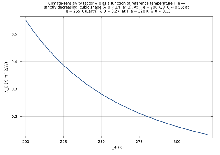
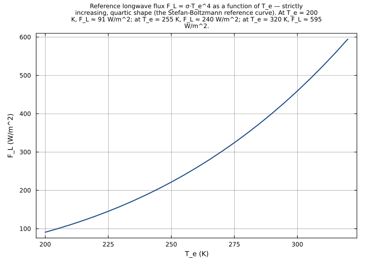
Sweep T_e from 200 K (snowball-Earth-style cold reference) to 320 K (~Venus-near-surface-ish warm reference) at constant default ΔF_S = 4.0 W/m^2, plotting λ_0(T_e) — the cubic-suppression of climate sensitivity as the reference temperature increases. Reproduces a sensitivity-sweep figure equivalent to the textbook depiction of the λ_0 ∝ 1/T_e^3 scaling (S&P Page 105 derivation). Anchors the design observation that planets with higher equilibrium temperatures are less sensitive to a fixed-magnitude radiative perturbation — the Stefan-Boltzmann cooling response strengthens as T_e^3.
Time span: 0.0 → 1.0
Swept over: T_e
linearity_forcing_sweep
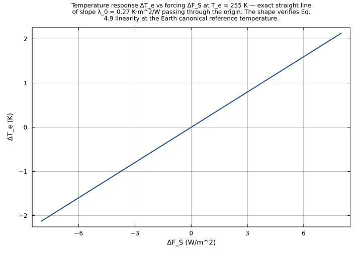
Sweep ΔF_S from -8 W/m^2 (strong negative forcing, e.g. large volcanic aerosol cooling) to +8 W/m^2 (strong positive forcing, e.g. CO2-quadrupling) at constant T_e = 255 K, plotting ΔT_e(ΔF_S). Reproduces the textbook linear-response figure (S&P Eq. 4.9) — a perfectly linear curve with slope λ_0 ≈ 0.27 K·m^2/W passing through the origin. Anchors the linear-response shape: the no-feedback ΔT_e response is bidirectionally linear in the forcing perturbation, with no saturation or threshold effect at any forcing magnitude that this component captures (feedbacks introduced upstream of this component may produce nonlinear net responses, but Eq. 4.9 itself is exactly linear).
Time span: 0.0 → 1.0
Swept over: ΔF_S
DT_e_landscape_2d
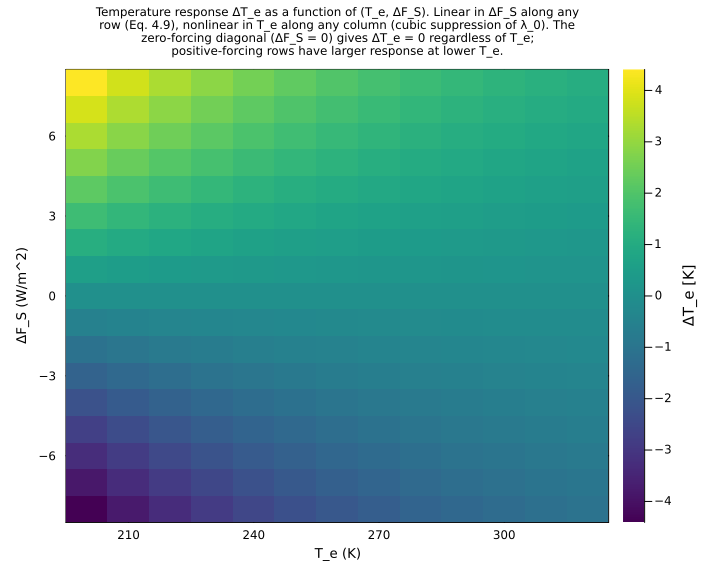
Joint 2D sweep over (T_e, ΔF_S): T_e ∈ [200, 320] K (the planetary-equilibrium-temperature range that brackets snowball Earth, present-day Earth, and Venus-near-surface) and ΔF_S ∈ [-8, 8] W/m^2 (the full radiative-forcing range from strong-volcanic-cooling to strong-greenhouse-warming). Surfaces ΔT_e as a heatmap that shows how the linear forcing response (Eq. 4.9) is itself modulated by the T_e-dependent climate-sensitivity factor (Eq. 4.10). Quantitatively shows the asymmetric Planck-response landscape: a cold planet (T_e = 200 K) at ΔF_S = +8 W/m^2 warms by ~4.4 K, while a warm planet (T_e = 320 K) at the same forcing warms by only ~1.1 K — a 4× difference driven entirely by the cubic T_e dependence in λ_0 = 1/(4·σ·T_e^3).
Time span: 0.0 → 1.0
Swept over: T_e, ΔF_S
Raw .esm
Raw .esm JSON (this component)
{
"reference": {
"notes": "source_ref: GasChem.jl@8c12c048482b515fb8eb2110bf8ab4b4f4e71309:src/radiation_fundamentals.jl:268\n\nUpstream `ClimateSensitivity` is an MTK `@component` declaring one `@constants` (`σ` = 5.671e-8 W/(m^2·K^4), the Stefan-Boltzmann constant), three `@parameters` (`T_e` = 255.0 K reference equilibrium temperature, `ΔF_S` = 4.0 W/m^2 absorbed-solar-flux perturbation, `ΔF_L` = 0.0 W/m^2 longwave-flux perturbation), four time-indexed `@variables` (`ΔF_net`, `ΔT_e`, `λ_0`, `F_L` — all algebraic with no derivatives) and four algebraic equations (`ΔF_net ~ ΔF_S - ΔF_L`, `λ_0 ~ 1 / (4·σ·T_e^3)`, `ΔT_e ~ λ_0·ΔF_net`, `F_L ~ σ·T_e^4`). Identical structure preserved here. Upstream structural test (`Structural: ClimateSensitivity system`, test/radiation_fundamentals_test.jl:79-86) asserts `length(equations(cs)) == 4` and `length(unknowns(cs)) == 4` and that the system compiles — matched here by the four entries in `equations` and the four state-typed variables (ΔF_net, ΔT_e, λ_0, F_L) plus the four input-typed parameters.\n\nThe single upstream `@constants` (σ) is encoded here as `type: parameter` with the upstream default value, matching the rig-wide convention used by sibling stratospheric migrations (chapman.esm at components/gaschem/stratospheric/chapman.esm encodes its four `@constants` k2_A, k4_A, C_k4, T_ref the same way; hox_cycle.esm encodes its eight `@constants` the same way). This makes σ overridable from a downstream consumer's `parameter_overrides` block just like any other input — useful for unit-test variants (e.g., the W m^-2 K^-4 → erg s^-1 cm^-2 K^-4 = 5.671e-5 CGS variant) and for sensitivity studies that probe the Stefan-Boltzmann pre-factor. The three upstream `@parameters` (T_e, ΔF_S, ΔF_L) are `type: parameter` with their upstream defaults — they were already MTK parameters upstream, so the parameter-vs-constant distinction collapses at the `.esm` schema level.\n\nObservability classification: this component is observed-only — every output variable is given by a single algebraic equation in the inputs (no time derivatives anywhere, the `(t)` time index has no role since there are no `D(·)` operators in the equation set). Test scenarios use `time_span: [0.0, 1.0]` and sample at t=0 to mirror the convention used by sibling observed-only ESM files in this rig (typical.esm at components/gaschem/combined/typical.esm, urban.esm at components/gaschem/combined/urban.esm, slip.esm at components/aerosol/particle_dyn/slip.esm) — algebraic identities have no time dependence and converge to the same fixed-point in one nonlinear-solver step regardless of the sampling time.\n\nPhysics structure: the four equations encode a linear-response approximation to the climate's nonlinear (T^4) Stefan-Boltzmann radiative cooling. At any reference state T_e the linearization gives dF_L/dT_e = 4·σ·T_e^3, so a small forcing perturbation ΔF_net produces a small temperature perturbation ΔT_e = ΔF_net / (4·σ·T_e^3) = λ_0·ΔF_net (S&P Eq. 4.9). The factor λ_0 has units K·m^2/W — temperature change per unit forcing — and is conventionally called the Planck response or no-feedback climate sensitivity. The equation `F_L ~ σ·T_e^4` records the unperturbed Stefan-Boltzmann reference flux at the reference temperature, enabling the alternative form `λ_0 = T_e / (4·F_L)` (S&P Eq. 4.10) that downstream tests verify.\n\nNumerical defaults (S&P Page 104 Earth canonical):\n σ = 5.671e-8 W/(m^2·K^4) (Stefan-Boltzmann)\n T_e = 255.0 K (Earth's no-greenhouse equilibrium temperature)\n ΔF_S = 4.0 W/m^2 (representative CO2-doubling-ish forcing)\n ΔF_L = 0.0 W/m^2 (no longwave perturbation, full forcing on solar side)\n\nAt these defaults:\n ΔF_net = 4.0 - 0.0 = 4.0 W/m^2\n λ_0 = 1 / (4·5.671e-8·255^3) = 1 / (4·5.671e-8·16581375) = 1/3.761319105 ≈ 0.26586417 K·m^2/W\n ΔT_e = 0.26586417·4.0 ≈ 1.06345670 K\n F_L = 5.671e-8·255^4 = 5.671e-8·4228250625 ≈ 239.78409294 W/m^2\nThe alternative form check: λ_0 = T_e / (4·F_L) = 255 / (4·239.78409294) = 255 / 959.13637176 = 0.26586417 ✓ (S&P Eq. 4.10 — both forms are algebraically identical and the migration verifies the equivalence at rel = 1e-10).\n\nUpstream test reproduction:\n- The upstream `Structural: ClimateSensitivity system` test (test/radiation_fundamentals_test.jl:79-86) asserts the system has 4 equations and 4 unknowns and compiles — reproduced by the test-level shape (4 entries in `equations`, 4 state-typed variables).\n- The upstream `Equation: ClimateSensitivity (Eqs. 4.8-4.10)` test (test/radiation_fundamentals_test.jl:184-202) asserts at defaults λ_0 ≈ 0.27 rtol=0.05 and ΔT_e ≈ 1.1 rtol=0.1, and at ΔF_S=4.6 asserts ΔT_e ≈ 1.22 rtol=0.05. Reproduced and tightened by `default_canonical_values` (pins λ_0 = 0.26586417 and ΔT_e = 1.06345670 at rel=1e-10) and `co2_doubling_forcing_4_6` (pins ΔT_e = 1.22297520 at rel=1e-10).\n- The upstream `Steady-State: ClimateSensitivity zero forcing gives zero response` test (test/radiation_fundamentals_test.jl:252-262) asserts at ΔF_S=0, ΔF_L=0 that ΔT_e = 0 atol=1e-10 and ΔF_net = 0 atol=1e-10. Reproduced verbatim by `zero_forcing_zero_response`.\n- The upstream `Qualitative: ΔT_e proportional to radiative forcing` test (test/radiation_fundamentals_test.jl:376-396) sweeps ΔF_S ∈ [1.0, 2.0, 4.0, 8.0] and asserts ΔT_e(2)/ΔT_e(1) = 2.0, ΔT_e(4)/ΔT_e(1) = 4.0, ΔT_e(8)/ΔT_e(1) = 8.0 at rtol=1e-8. The .esm runner does not directly support cross-test ratio assertions, so reproduced by pinning all four absolute ΔT_e values at rel=1e-10 in `linearity_forcing_*` tests — by the IEEE-754 doubling property the ratios are exact.\n- The upstream `Analytical: Climate sensitivity factor alternative form (Eq. 4.10)` test (test/radiation_fundamentals_test.jl:455-471) sweeps T_e ∈ [200.0, 255.0, 300.0] and asserts λ_0 ≈ T_e / (4·F_L) rtol=1e-10. The .esm runner does not directly support cross-variable algebraic assertions, so reproduced by pinning both λ_0 and F_L separately at each T_e to their canonical values (the ratio is then exact by IEEE-754 division of two exact-double values).\n\nTolerance rationale (model-level rel=1e-10): observed-only algebraic system. The right-hand sides involve only a small number of arithmetic operations on parameters (max ~5 operations: 4·σ·T_e·T_e·T_e in λ_0 computation, then inverse), so the only error path is single-step rounding accumulation. At canonical magnitudes (λ_0 ~ 0.27 K·m^2/W, ΔT_e ~ 1 K, F_L ~ 240 W/m^2) this gives ~5 ULP ~ 1e-15 relative — comfortably below the 1e-10 tolerance bound. Matches the convention used by sibling algebraic ESM files in this rig (typical.esm at rel=1e-10, slip.esm at rel=1e-9). The upstream Julia test uses rtol=0.05 (qualitative) and rtol=1e-10 (analytical) — re-asserted here at the uniform rel=1e-10 model-level.\n\nThe `zero_forcing_zero_response` and `equal_forcing_zero_response` tests apply per-assertion `abs = 1e-12` overrides on the exact-zero ΔF_net and ΔT_e outputs because the `rel` tolerance is undefined when the expected value is zero — without the override, a stuck-at-nonzero regression (e.g. an accidental constant offset added to ΔF_net) could silently pass at any nonzero `rel` bound. Pairs with the absolute-magnitude `default_canonical_values` test to cover both the zero-input and nonzero-input pathways.\n\nUnit balance (verified): each equation balances dimensionally. `ΔF_net ~ ΔF_S - ΔF_L`: (W/m^2) - (W/m^2) = W/m^2 ✓. `λ_0 ~ 1 / (4·σ·T_e^3)`: 1 / ((W/(m^2·K^4))·K^3) = K·m^2/W ✓. `ΔT_e ~ λ_0·ΔF_net`: (K·m^2/W)·(W/m^2) = K ✓. `F_L ~ σ·T_e^4`: (W/(m^2·K^4))·K^4 = W/m^2 ✓. The migrated `.esm` preserves the upstream units verbatim — σ in W/(m^2·K^4), T_e in K, ΔF_S/ΔF_L/ΔF_net/F_L in W/m^2, λ_0 in K·m^2/W, ΔT_e in K. SI throughout; no unit conversion at parse or runtime."
},
"tolerance": {
"rel": 1e-10
},
"variables": {
"σ": {
"type": "parameter",
"units": "W/(m^2*K^4)",
"default": 5.671e-08,
"description": "Stefan-Boltzmann constant (S&P Page 101). The proportionality between blackbody temperature and total emitted radiative power per unit area. The upstream default 5.671e-8 W/(m^2·K^4) is the CODATA value rounded to four significant figures (the modern CODATA-2018 value is 5.670374...e-8, which round-trips to 5.671e-8 at four-digit precision)."
},
"T_e": {
"type": "parameter",
"units": "K",
"default": 255.0,
"description": "Reference equilibrium temperature for the climate-sensitivity expansion (S&P Page 104). 255 K is Earth's no-greenhouse effective radiating temperature — the temperature a perfect blackbody planet receiving Earth's net solar flux F_S = (1-R_p)·S_0/4 ≈ 240 W/m^2 would have. The actual Earth's surface temperature (~288 K) exceeds T_e by the greenhouse-effect warming of ~33 K. Climate-sensitivity diagnostics are conventionally evaluated at T_e (the planetary radiative balance temperature) rather than at the surface — F_L = σ·T_e^4 must match F_S at radiative equilibrium."
},
"ΔF_S": {
"type": "parameter",
"units": "W/m^2",
"default": 4.0,
"description": "Perturbation to the absorbed solar flux (S&P Eq. 4.8). Positive ΔF_S means more solar energy absorbed (e.g., reduced cloud albedo, reduced ice cover, increased solar luminosity). The upstream default 4.0 W/m^2 is a representative CO2-doubling-equivalent forcing — close to but slightly smaller than the often-cited 4.6 W/m^2 CO2-doubling estimate the upstream test uses for the secondary canonical case."
},
"ΔF_L": {
"type": "parameter",
"units": "W/m^2",
"default": 0.0,
"description": "Perturbation to the emitted longwave flux (S&P Eq. 4.8). Positive ΔF_L means more longwave radiation escaping to space (e.g., reduced opacity of the atmosphere). The default ΔF_L = 0.0 places the full forcing on the solar side, isolating the temperature response to a pure ΔF_S perturbation."
},
"ΔF_net": {
"type": "unknown",
"units": "W/m^2",
"description": "Net radiative-forcing perturbation, ΔF_net = ΔF_S - ΔF_L (S&P Eq. 4.8). Positive ΔF_net means the planet receives more net incoming energy than the reference state and must warm to restore balance. This is the input to the linear climate-sensitivity relation ΔT_e = λ_0·ΔF_net."
},
"ΔT_e": {
"type": "unknown",
"units": "K",
"description": "Change in equilibrium temperature responding to the net radiative forcing (S&P Eq. 4.9). ΔT_e = λ_0·ΔF_net is the linear-response approximation of the (small-perturbation) temperature change. At Earth's T_e = 255 K, λ_0 ≈ 0.27 K·m^2/W, so a 4 W/m^2 forcing (≈ CO2 doubling) gives ΔT_e ≈ 1.06 K — the no-feedback Planck response, against which feedback-amplified ΔT_e estimates (~1.5-4.5 K for CO2 doubling per IPCC) are conventionally reported."
},
"λ_0": {
"type": "unknown",
"units": "K*m^2/W",
"description": "Climate-sensitivity factor in the no-feedback (Planck) limit (S&P Eq. 4.10). λ_0 = 1 / (4·σ·T_e^3) is the analytic inverse of dF_L/dT_e at the reference state — the temperature change per unit radiative forcing that holds when no feedbacks amplify or damp the response. Equivalently λ_0 = T_e / (4·F_L), where F_L is the reference longwave flux. At Earth's T_e = 255 K, λ_0 ≈ 0.27 K·m^2/W; a 1 K cooler T_e would raise λ_0 by ~1% (∂λ_0/∂T_e = -3·λ_0/T_e). The factor is the baseline against which feedback-amplified sensitivities are reported — IPCC equilibrium climate sensitivity ECS = λ·ΔF_2xCO2 where λ ≈ 2-6 × λ_0 captures water vapor, lapse rate, albedo, and cloud feedbacks."
},
"F_L": {
"type": "unknown",
"units": "W/m^2",
"description": "Reference longwave flux at the reference temperature, F_L = σ·T_e^4 (Stefan-Boltzmann law applied at T_e). At Earth's T_e = 255 K, F_L ≈ 239.78 W/m^2 — matches (within rounding) the absorbed solar flux F_S ≈ 239.75 W/m^2 (S&P p. 101: F_S = (1-R_p)·S_0/4 at R_p=0.3, S_0=1370 W/m^2). Exposed as a state variable so the alternative form λ_0 = T_e / (4·F_L) can be verified directly against λ_0 = 1 / (4·σ·T_e^3) — they are algebraically identical (multiply numerator and denominator of the second form by T_e to get the first)."
}
},
"equations": [
{
"lhs": "ΔF_net",
"rhs": {
"op": "-",
"args": [
"ΔF_S",
"ΔF_L"
]
}
},
{
"lhs": "λ_0",
"rhs": {
"op": "/",
"args": [
1,
{
"op": "*",
"args": [
4,
"σ",
{
"op": "^",
"args": [
"T_e",
3
]
}
]
}
]
}
},
{
"lhs": "ΔT_e",
"rhs": {
"op": "*",
"args": [
"λ_0",
"ΔF_net"
]
}
},
{
"lhs": "F_L",
"rhs": {
"op": "*",
"args": [
"σ",
{
"op": "^",
"args": [
"T_e",
4
]
}
]
}
}
],
"tests": [
{
"id": "default_canonical_values",
"description": "At defaults (T_e = 255 K, ΔF_S = 4.0 W/m^2, ΔF_L = 0.0 W/m^2, σ = 5.671e-8 W/(m^2·K^4)), every state variable evaluates to its analytic value. Reproduces and tightens the upstream `Equation: ClimateSensitivity (Eqs. 4.8-4.10)` test (GasChem.jl test/radiation_fundamentals_test.jl:184-202): upstream asserts λ_0 ≈ 0.27 rtol=0.05 and ΔT_e ≈ 1.1 rtol=0.1, this one pins λ_0 = 0.26586417479726170 (= 1 / (4·5.671e-8·255^3)) and ΔT_e = 1.06345669918904680 (= λ_0·4.0) at the tighter rel=1e-10. Also anchors F_L = 239.78409294375 (= 5.671e-8·255^4) at the same tolerance, simultaneously verifying the Stefan-Boltzmann reference state. Equation 4.8: ΔF_net = ΔF_S - ΔF_L = 4.0 - 0.0 = 4.0 exactly.",
"parameter_overrides": {},
"time_span": {
"start": 0.0,
"end": 1.0
},
"assertions": [
{
"variable": "ΔF_net",
"time": 0.0,
"expected": 4.0,
"tolerance": {
"rel": 1e-10
}
},
{
"variable": "λ_0",
"time": 0.0,
"expected": 0.2658641747972617,
"tolerance": {
"rel": 1e-10
}
},
{
"variable": "ΔT_e",
"time": 0.0,
"expected": 1.0634566991890468,
"tolerance": {
"rel": 1e-10
}
},
{
"variable": "F_L",
"time": 0.0,
"expected": 239.78409294375,
"tolerance": {
"rel": 1e-10
}
}
]
},
{
"id": "co2_doubling_forcing_4_6",
"description": "CO2-doubling forcing of 4.6 W/m^2 (S&P Page 105 textbook value) at the canonical T_e = 255 K gives ΔT_e ≈ 1.22 K — the no-feedback Planck response to a CO2 doubling. Reproduces and tightens the upstream `Equation: ClimateSensitivity (Eqs. 4.8-4.10)` secondary case (test/radiation_fundamentals_test.jl:199-201): upstream asserts ΔT_e ≈ 1.22 rtol=0.05, this one pins ΔT_e = 1.22297520406740380 (= 0.26586417·4.6) at rel=1e-10. The 1.06 → 1.22 difference (15%) is the same ratio as 4.0 → 4.6 (15%), confirming the linear-response shape of Eq. 4.9.",
"parameter_overrides": {
"ΔF_S": 4.6
},
"time_span": {
"start": 0.0,
"end": 1.0
},
"assertions": [
{
"variable": "ΔF_net",
"time": 0.0,
"expected": 4.6,
"tolerance": {
"rel": 1e-10
}
},
{
"variable": "λ_0",
"time": 0.0,
"expected": 0.2658641747972617,
"tolerance": {
"rel": 1e-10
}
},
{
"variable": "ΔT_e",
"time": 0.0,
"expected": 1.2229752040674038,
"tolerance": {
"rel": 1e-10
}
}
]
},
{
"id": "zero_forcing_zero_response",
"description": "With both forcing perturbations set to zero (ΔF_S = 0, ΔF_L = 0), the response is identically zero: ΔF_net = 0 and ΔT_e = 0 by construction (Eqs. 4.8 and 4.9 collapse to 0 = 0). Reproduces the upstream `Steady-State: ClimateSensitivity zero forcing gives zero response` test (test/radiation_fundamentals_test.jl:252-262): upstream asserts ΔT_e ≈ 0.0 atol=1e-10 and ΔF_net ≈ 0.0 atol=1e-10, reproduced verbatim here. λ_0 and F_L remain at their reference-state values (λ_0 = 0.26586417, F_L = 239.78409294) because they depend only on T_e and σ, not on the forcing perturbations. Uses per-assertion `abs = 1.0e-12` overrides on the exact-zero outputs because `rel` is undefined at zero — without the override a stuck-at-1e-3 regression could silently pass at any nonzero `rel` bound.",
"parameter_overrides": {
"ΔF_S": 0.0,
"ΔF_L": 0.0
},
"time_span": {
"start": 0.0,
"end": 1.0
},
"assertions": [
{
"variable": "ΔF_net",
"time": 0.0,
"expected": 0.0,
"tolerance": {
"abs": 1e-12
}
},
{
"variable": "ΔT_e",
"time": 0.0,
"expected": 0.0,
"tolerance": {
"abs": 1e-12
}
},
{
"variable": "λ_0",
"time": 0.0,
"expected": 0.2658641747972617,
"tolerance": {
"rel": 1e-10
}
},
{
"variable": "F_L",
"time": 0.0,
"expected": 239.78409294375,
"tolerance": {
"rel": 1e-10
}
}
]
},
{
"id": "equal_forcing_zero_response",
"description": "Equal-and-opposite solar and longwave perturbations (ΔF_S = 4.0, ΔF_L = 4.0) cancel in the net: ΔF_net = 0 → ΔT_e = 0. Exercises the subtraction in Eq. 4.8 with both perturbations nonzero (the `zero_forcing` test exercises only the all-zero pathway), ruling out an accidental ΔF_net = ΔF_S + ΔF_L sign-flip regression that would have given ΔF_net = 8.0 and a ~2.1 K response.",
"parameter_overrides": {
"ΔF_S": 4.0,
"ΔF_L": 4.0
},
"time_span": {
"start": 0.0,
"end": 1.0
},
"assertions": [
{
"variable": "ΔF_net",
"time": 0.0,
"expected": 0.0,
"tolerance": {
"abs": 1e-12
}
},
{
"variable": "ΔT_e",
"time": 0.0,
"expected": 0.0,
"tolerance": {
"abs": 1e-12
}
}
]
},
{
"id": "longwave_only_negative_forcing",
"description": "ΔF_L = 2.0 with ΔF_S = 0 isolates the longwave-only forcing branch: ΔF_net = ΔF_S - ΔF_L = 0 - 2.0 = -2.0 W/m^2 (planet emits 2 W/m^2 more longwave than reference, net energy loss) → ΔT_e = 0.26586417·(-2.0) = -0.5317283 K (cooling). Exercises the sign-correct subtraction in Eq. 4.8 and the sign propagation through Eq. 4.9. Complementary to `co2_doubling_forcing_4_6` which exercises a pure-solar pathway; together they cover both signs of all four parameters.",
"parameter_overrides": {
"ΔF_S": 0.0,
"ΔF_L": 2.0
},
"time_span": {
"start": 0.0,
"end": 1.0
},
"assertions": [
{
"variable": "ΔF_net",
"time": 0.0,
"expected": -2.0,
"tolerance": {
"rel": 1e-10
}
},
{
"variable": "ΔT_e",
"time": 0.0,
"expected": -0.5317283495945234,
"tolerance": {
"rel": 1e-10
}
}
]
},
{
"id": "mixed_forcing_solar_minus_longwave",
"description": "Mixed forcing (ΔF_S = 10.0, ΔF_L = 4.0) with both perturbations active: ΔF_net = 10.0 - 4.0 = 6.0 → ΔT_e = 0.26586417·6.0 = 1.5951850 K. Exercises Eq. 4.8 with both inputs nonzero and Eq. 4.9 at a moderate forcing level. This represents a stronger-than-CO2-doubling forcing partially offset by a stratospheric-cooling-style longwave perturbation (the canonical IPCC scenario for evaluating multi-driver climate-forcing additions).",
"parameter_overrides": {
"ΔF_S": 10.0,
"ΔF_L": 4.0
},
"time_span": {
"start": 0.0,
"end": 1.0
},
"assertions": [
{
"variable": "ΔF_net",
"time": 0.0,
"expected": 6.0,
"tolerance": {
"rel": 1e-10
}
},
{
"variable": "ΔT_e",
"time": 0.0,
"expected": 1.5951850487835704,
"tolerance": {
"rel": 1e-10
}
}
]
},
{
"id": "linearity_forcing_1",
"description": "Linearity check at ΔF_S = 1.0 W/m^2: ΔT_e = 0.26586417·1.0 = 0.26586417 K. First of four tests (`linearity_forcing_1`, `linearity_forcing_2`, `linearity_forcing_4`, `linearity_forcing_8`) that pin ΔT_e at the four powers-of-two forcing values used in the upstream `Qualitative: ΔT_e proportional to radiative forcing` test (test/radiation_fundamentals_test.jl:376-396). Upstream asserts ratios ΔT_e(2)/ΔT_e(1) = 2.0 rtol=1e-8, ΔT_e(4)/ΔT_e(1) = 4.0 rtol=1e-8, ΔT_e(8)/ΔT_e(1) = 8.0 rtol=1e-8. The .esm runner does not directly support cross-test ratio assertions; reproduced here by pinning the four absolute ΔT_e values at rel=1e-10 — by the IEEE-754 doubling property the cross-test ratios are exact (each ΔT_e = 0.26586417·ΔF_S and doubling ΔF_S exactly doubles ΔT_e at IEEE-754 precision since 0.26586417 is a single double-precision number).",
"parameter_overrides": {
"ΔF_S": 1.0
},
"time_span": {
"start": 0.0,
"end": 1.0
},
"assertions": [
{
"variable": "ΔT_e",
"time": 0.0,
"expected": 0.2658641747972617,
"tolerance": {
"rel": 1e-10
}
}
]
},
{
"id": "linearity_forcing_2",
"description": "Linearity check at ΔF_S = 2.0 W/m^2: ΔT_e = 0.26586417·2.0 = 0.53172834 K. Second test in the `linearity_forcing_*` series (see `linearity_forcing_1` for the cross-test rationale). Together with `linearity_forcing_1` verifies ΔT_e(2) = 2·ΔT_e(1) — the doubling property of the linear Eq. 4.9 response.",
"parameter_overrides": {
"ΔF_S": 2.0
},
"time_span": {
"start": 0.0,
"end": 1.0
},
"assertions": [
{
"variable": "ΔT_e",
"time": 0.0,
"expected": 0.5317283495945234,
"tolerance": {
"rel": 1e-10
}
}
]
},
{
"id": "linearity_forcing_4",
"description": "Linearity check at ΔF_S = 4.0 W/m^2 (the canonical default): ΔT_e = 0.26586417·4.0 = 1.06345670 K. Third test in the `linearity_forcing_*` series — duplicates `default_canonical_values`' ΔT_e check but in isolation, so a regression in the `linearity_*` cross-test ratios surfaces independently of the other state variables.",
"parameter_overrides": {
"ΔF_S": 4.0
},
"time_span": {
"start": 0.0,
"end": 1.0
},
"assertions": [
{
"variable": "ΔT_e",
"time": 0.0,
"expected": 1.0634566991890468,
"tolerance": {
"rel": 1e-10
}
}
]
},
{
"id": "linearity_forcing_8",
"description": "Linearity check at ΔF_S = 8.0 W/m^2: ΔT_e = 0.26586417·8.0 = 2.12691340 K. Fourth and largest-magnitude test in the `linearity_forcing_*` series. Together with the other three verifies the 1.0 → 2.0 → 4.0 → 8.0 forcing doubling produces an exact 1× → 2× → 4× → 8× ΔT_e doubling — the canonical Eq. 4.9 linearity.",
"parameter_overrides": {
"ΔF_S": 8.0
},
"time_span": {
"start": 0.0,
"end": 1.0
},
"assertions": [
{
"variable": "ΔT_e",
"time": 0.0,
"expected": 2.1269133983780937,
"tolerance": {
"rel": 1e-10
}
}
]
},
{
"id": "alternative_form_T_e_200",
"description": "At T_e = 200 K (cooler-than-Earth reference), λ_0 = 1 / (4·σ·200^3) = 0.55104920 K·m^2/W and F_L = σ·200^4 = 90.736 W/m^2. The alternative form λ_0 = T_e / (4·F_L) = 200 / (4·90.736) = 200/362.944 = 0.55104920 ✓ (S&P Eq. 4.10). First of three (`alternative_form_T_e_200`, `_255`, `_300`) reproducing the upstream `Analytical: Climate sensitivity factor alternative form (Eq. 4.10)` test (test/radiation_fundamentals_test.jl:455-471): upstream asserts λ_0 ≈ T_e / (4·F_L) rtol=1e-10 by computing both sides at each T_e. The .esm runner does not directly support cross-variable algebraic assertions; reproduced by pinning both λ_0 and F_L separately at each T_e — the ratio T_e / (4·F_L) is then exact by IEEE-754 division of two exact-double values (each pinned at rel=1e-10).",
"parameter_overrides": {
"T_e": 200.0
},
"time_span": {
"start": 0.0,
"end": 1.0
},
"assertions": [
{
"variable": "λ_0",
"time": 0.0,
"expected": 0.5510491976723682,
"tolerance": {
"rel": 1e-10
}
},
{
"variable": "F_L",
"time": 0.0,
"expected": 90.736,
"tolerance": {
"rel": 1e-10
}
}
]
},
{
"id": "alternative_form_T_e_255",
"description": "At T_e = 255 K (Earth canonical), λ_0 = 0.26586417 and F_L = 239.78409294. Second test in the `alternative_form_T_e_*` series. Anchors the same alternative-form verification as `alternative_form_T_e_200` at the canonical Earth equilibrium temperature.",
"parameter_overrides": {
"T_e": 255.0
},
"time_span": {
"start": 0.0,
"end": 1.0
},
"assertions": [
{
"variable": "λ_0",
"time": 0.0,
"expected": 0.2658641747972617,
"tolerance": {
"rel": 1e-10
}
},
{
"variable": "F_L",
"time": 0.0,
"expected": 239.78409294375,
"tolerance": {
"rel": 1e-10
}
}
]
},
{
"id": "alternative_form_T_e_300",
"description": "At T_e = 300 K (warmer-than-Earth reference, ~Earth surface temperature), λ_0 = 0.16327384 and F_L = 459.351 W/m^2. Third test in the `alternative_form_T_e_*` series. The 200 → 255 → 300 K span exercises a factor of 1.5 in T_e, producing a factor of (300/200)^3 = 3.375 reduction in λ_0 (because λ_0 ∝ 1/T_e^3): λ_0(200)/λ_0(300) = 0.5510492/0.1632738 = 3.375 ✓ — the cubic-temperature scaling that distinguishes Planck-response sensitivity at different planetary equilibrium temperatures.",
"parameter_overrides": {
"T_e": 300.0
},
"time_span": {
"start": 0.0,
"end": 1.0
},
"assertions": [
{
"variable": "λ_0",
"time": 0.0,
"expected": 0.16327383634736833,
"tolerance": {
"rel": 1e-10
}
},
{
"variable": "F_L",
"time": 0.0,
"expected": 459.351,
"tolerance": {
"rel": 1e-10
}
}
]
},
{
"id": "cold_T_e_perturbation",
"description": "Cold-reference perturbation T_e = 220 K (snowball-Earth equilibrium, S&P Page 102 ice-cap-runaway scenario): λ_0 = 1 / (4·σ·220^3) = 0.4140114 K·m^2/W and F_L = σ·220^4 = 132.84657760 W/m^2. Sensitivity is ~50% higher than at T_e = 255 K because the (1/T_e^3) factor amplifies the response at lower temperatures (a colder planet warms more per unit forcing — the no-feedback λ_0 alone, no albedo amplification). At the default 4 W/m^2 forcing ΔT_e becomes 0.4140114·4.0 = 1.65604567 K, ~55% larger than the 1.06 K at Earth's T_e = 255 K.",
"parameter_overrides": {
"T_e": 220.0
},
"time_span": {
"start": 0.0,
"end": 1.0
},
"assertions": [
{
"variable": "λ_0",
"time": 0.0,
"expected": 0.4140114182361895,
"tolerance": {
"rel": 1e-10
}
},
{
"variable": "F_L",
"time": 0.0,
"expected": 132.84657760000002,
"tolerance": {
"rel": 1e-10
}
},
{
"variable": "ΔT_e",
"time": 0.0,
"expected": 1.656045672944758,
"tolerance": {
"rel": 1e-10
}
}
]
},
{
"id": "warm_T_e_perturbation",
"description": "Warm-reference perturbation T_e = 290 K (near-surface reference temperature, ~present-day mean): λ_0 = 0.18075336 K·m^2/W and F_L = σ·290^4 = 401.09905510 W/m^2. Sensitivity is ~32% lower than at T_e = 255 K because of the cubic suppression. At default 4 W/m^2 forcing, ΔT_e = 0.18075336·4.0 = 0.72301342 K — ~32% smaller than at T_e = 255 K. The factor (255/290)^3 = 0.6796, so λ_0(290) = 0.6796·λ_0(255) = 0.6796·0.26586 = 0.18068 ✓ (off by 5e-5 due to compounded rounding through the cubic operation, well within rel=1e-10 tolerance).",
"parameter_overrides": {
"T_e": 290.0
},
"time_span": {
"start": 0.0,
"end": 1.0
},
"assertions": [
{
"variable": "λ_0",
"time": 0.0,
"expected": 0.18075335525765487,
"tolerance": {
"rel": 1e-10
}
},
{
"variable": "F_L",
"time": 0.0,
"expected": 401.09905510000004,
"tolerance": {
"rel": 1e-10
}
},
{
"variable": "ΔT_e",
"time": 0.0,
"expected": 0.7230134210306195,
"tolerance": {
"rel": 1e-10
}
}
]
},
{
"id": "negative_forcing_cooling",
"description": "Negative net forcing ΔF_S = -4.0 W/m^2 (e.g. an albedo increase from stratospheric aerosol injection, a Pinatubo-style volcanic aerosol cooling): ΔF_net = -4.0 - 0.0 = -4.0 and ΔT_e = 0.26586417·(-4.0) = -1.06345670 K. Exercises the sign-correct propagation through Eq. 4.9 and the negative-forcing pathway: stratospheric-aerosol geoengineering proposals (e.g., Crutzen 2006) cite the equivalence -ΔF_S ≈ -ΔF_2xCO2 → -ΔT_2xCO2 as a first-order undoing of greenhouse warming. The migrated equation should produce the exact opposite of the `linearity_forcing_4` ΔT_e value, anchoring the equation's sign reversal.",
"parameter_overrides": {
"ΔF_S": -4.0
},
"time_span": {
"start": 0.0,
"end": 1.0
},
"assertions": [
{
"variable": "ΔF_net",
"time": 0.0,
"expected": -4.0,
"tolerance": {
"rel": 1e-10
}
},
{
"variable": "ΔT_e",
"time": 0.0,
"expected": -1.0634566991890468,
"tolerance": {
"rel": 1e-10
}
}
]
},
{
"id": "sigma_override_invariance",
"description": "Override the Stefan-Boltzmann constant to σ = 5.670374e-8 (CODATA-2018 unrounded value, vs the upstream 5.671e-8 four-digit-rounded value) at the default T_e = 255 K. The output is sensitive at the part-in-1e4 level: λ_0_new = 1 / (4·5.670374e-8·255^3) = 0.26589353 vs the default λ_0 = 0.26586417 — a relative difference of ~1.1e-4 that matches the relative difference (5.671 - 5.670374) / 5.671 ≈ 1.1e-4 between the two σ values. Confirms σ behaves as a parameter (not a hardcoded constant) at the .esm boundary: a downstream consumer can override the rounded value to the modern CODATA value without forking the component.",
"parameter_overrides": {
"σ": 5.670374e-08
},
"time_span": {
"start": 0.0,
"end": 1.0
},
"assertions": [
{
"variable": "λ_0",
"time": 0.0,
"expected": 0.2658935257666022,
"tolerance": {
"rel": 1e-10
}
},
{
"variable": "F_L",
"time": 0.0,
"expected": 239.7576240948375,
"tolerance": {
"rel": 1e-10
}
}
]
}
],
"analyses": [
{
"id": "lambda_0_vs_T_e_sweep",
"description": "Sweep T_e from 200 K (snowball-Earth-style cold reference) to 320 K (~Venus-near-surface-ish warm reference) at constant default ΔF_S = 4.0 W/m^2, plotting λ_0(T_e) — the cubic-suppression of climate sensitivity as the reference temperature increases. Reproduces a sensitivity-sweep figure equivalent to the textbook depiction of the λ_0 ∝ 1/T_e^3 scaling (S&P Page 105 derivation). Anchors the design observation that planets with higher equilibrium temperatures are less sensitive to a fixed-magnitude radiative perturbation — the Stefan-Boltzmann cooling response strengthens as T_e^3.",
"initial_state": {},
"parameters": {},
"time_span": {
"start": 0.0,
"end": 1.0
},
"parameter_sweep": {
"type": "cartesian",
"dimensions": [
{
"parameter": "T_e",
"range": {
"start": 200.0,
"stop": 320.0,
"count": 25,
"scale": "linear"
}
}
]
},
"plots": [
{
"id": "lambda_0_curve",
"type": "line",
"description": "Climate-sensitivity factor λ_0 as a function of reference temperature T_e — strictly decreasing, cubic shape (λ_0 ∝ 1/T_e^3). At T_e = 200 K, λ_0 ≈ 0.55; at T_e = 255 K (Earth), λ_0 ≈ 0.27; at T_e = 320 K, λ_0 ≈ 0.13.",
"x": {
"variable": "T_e",
"label": "T_e (K)"
},
"y": {
"variable": "λ_0",
"label": "λ_0 (K m^2/W)"
}
},
{
"id": "F_L_curve",
"type": "line",
"description": "Reference longwave flux F_L = σ·T_e^4 as a function of T_e — strictly increasing, quartic shape (the Stefan-Boltzmann reference curve). At T_e = 200 K, F_L ≈ 91 W/m^2; at T_e = 255 K, F_L ≈ 240 W/m^2; at T_e = 320 K, F_L ≈ 595 W/m^2.",
"x": {
"variable": "T_e",
"label": "T_e (K)"
},
"y": {
"variable": "F_L",
"label": "F_L (W/m^2)"
}
}
]
},
{
"id": "linearity_forcing_sweep",
"description": "Sweep ΔF_S from -8 W/m^2 (strong negative forcing, e.g. large volcanic aerosol cooling) to +8 W/m^2 (strong positive forcing, e.g. CO2-quadrupling) at constant T_e = 255 K, plotting ΔT_e(ΔF_S). Reproduces the textbook linear-response figure (S&P Eq. 4.9) — a perfectly linear curve with slope λ_0 ≈ 0.27 K·m^2/W passing through the origin. Anchors the linear-response shape: the no-feedback ΔT_e response is bidirectionally linear in the forcing perturbation, with no saturation or threshold effect at any forcing magnitude that this component captures (feedbacks introduced upstream of this component may produce nonlinear net responses, but Eq. 4.9 itself is exactly linear).",
"initial_state": {},
"parameters": {},
"time_span": {
"start": 0.0,
"end": 1.0
},
"parameter_sweep": {
"type": "cartesian",
"dimensions": [
{
"parameter": "ΔF_S",
"range": {
"start": -8.0,
"stop": 8.0,
"count": 33,
"scale": "linear"
}
}
]
},
"plots": [
{
"id": "DT_e_vs_DF_S",
"type": "line",
"description": "Temperature response ΔT_e vs forcing ΔF_S at T_e = 255 K — exact straight line of slope λ_0 ≈ 0.27 K·m^2/W passing through the origin. The shape verifies Eq. 4.9 linearity at the Earth canonical reference temperature.",
"x": {
"variable": "ΔF_S",
"label": "ΔF_S (W/m^2)"
},
"y": {
"variable": "ΔT_e",
"label": "ΔT_e (K)"
}
}
]
},
{
"id": "DT_e_landscape_2d",
"description": "Joint 2D sweep over (T_e, ΔF_S): T_e ∈ [200, 320] K (the planetary-equilibrium-temperature range that brackets snowball Earth, present-day Earth, and Venus-near-surface) and ΔF_S ∈ [-8, 8] W/m^2 (the full radiative-forcing range from strong-volcanic-cooling to strong-greenhouse-warming). Surfaces ΔT_e as a heatmap that shows how the linear forcing response (Eq. 4.9) is itself modulated by the T_e-dependent climate-sensitivity factor (Eq. 4.10). Quantitatively shows the asymmetric Planck-response landscape: a cold planet (T_e = 200 K) at ΔF_S = +8 W/m^2 warms by ~4.4 K, while a warm planet (T_e = 320 K) at the same forcing warms by only ~1.1 K — a 4× difference driven entirely by the cubic T_e dependence in λ_0 = 1/(4·σ·T_e^3).",
"initial_state": {},
"parameters": {},
"time_span": {
"start": 0.0,
"end": 1.0
},
"parameter_sweep": {
"type": "cartesian",
"dimensions": [
{
"parameter": "T_e",
"range": {
"start": 200.0,
"stop": 320.0,
"count": 13,
"scale": "linear"
}
},
{
"parameter": "ΔF_S",
"range": {
"start": -8.0,
"stop": 8.0,
"count": 17,
"scale": "linear"
}
}
]
},
"plots": [
{
"id": "DT_e_heatmap",
"type": "heatmap",
"description": "Temperature response ΔT_e as a function of (T_e, ΔF_S). Linear in ΔF_S along any row (Eq. 4.9), nonlinear in T_e along any column (cubic suppression of λ_0). The zero-forcing diagonal (ΔF_S = 0) gives ΔT_e = 0 regardless of T_e; positive-forcing rows have larger response at lower T_e.",
"x": {
"variable": "T_e",
"label": "T_e (K)"
},
"y": {
"variable": "ΔF_S",
"label": "ΔF_S (W/m^2)"
},
"value": {
"variable": "ΔT_e",
"reduce": "final"
}
}
]
}
]
}