OHProduction
Tropospheric OH radical production from O₃ photolysis — Seinfeld & Pandis (2006) Ch. 6 §6.1 Eqs. 6.1, 6.3, 6.4, pp. 204-207. The dominant source of OH in the troposphere is O₃ photolysis below 320 nm producing electronically excited O(¹D), which either reacts with H₂O to yield two OH radicals or is collisionally quenched back to ground-state O(³P) by N₂/O₂. Implements three algebraic relations: (Eq. 6.1) O(¹D) steady-state concentration [O(¹D)] = j_O₃·[O₃] / (k₃[M] + k₄[H₂O]), (Eq. 6.4) OH yield ε_OH = 2·k₄[H₂O] / (k₃[M] + k₄[H₂O]) as the fraction of O(¹D) producing OH (the factor of 2 accounts for the 2 OH produced per O(¹D)+H₂O encounter — ε_OH ranges 0..2), (Eq. 6.3) OH production rate P_OH = j_O₃·[O₃]·ε_OH. The effective quenching rate k₃_eff = f_N₂·k₃,N₂ + f_O₂·k₃,O₂ is the air-composition-weighted average of the N₂ and O₂ quenching channels. Observed-only algebraic system (no time derivatives): six variables (three inputs O₃/H₂O/M as parameters, three outputs O₁D/ε_OH/P_OH as state) plus six rate-parameter inputs (j_O₃, k₃_N₂, k₃_O₂, k₄, f_N₂, f_O₂) and one stoichiometric constant (two=2). Migrated from GasChem.jl@8c12c048 src/oh_production.jl:88 (`OHProduction` @component).
Description
Tropospheric OH radical production from O₃ photolysis — Seinfeld & Pandis (2006) Ch. 6 §6.1 Eqs. 6.1, 6.3, 6.4, pp. 204-207. The dominant source of OH in the troposphere is O₃ photolysis below 320 nm producing electronically excited O(¹D), which either reacts with H₂O to yield two OH radicals or is collisionally quenched back to ground-state O(³P) by N₂/O₂. Implements three algebraic relations: (Eq. 6.1) O(¹D) steady-state concentration [O(¹D)] = j_O₃·[O₃] / (k₃[M] + k₄[H₂O]), (Eq. 6.4) OH yield ε_OH = 2·k₄[H₂O] / (k₃[M] + k₄[H₂O]) as the fraction of O(¹D) producing OH (the factor of 2 accounts for the 2 OH produced per O(¹D)+H₂O encounter — ε_OH ranges 0..2), (Eq. 6.3) OH production rate P_OH = j_O₃·[O₃]·ε_OH. The effective quenching rate k₃_eff = f_N₂·k₃,N₂ + f_O₂·k₃,O₂ is the air-composition-weighted average of the N₂ and O₂ quenching channels. Observed-only algebraic system (no time derivatives): six variables (three inputs O₃/H₂O/M as parameters, three outputs O₁D/ε_OH/P_OH as state) plus six rate-parameter inputs (j_O₃, k₃_N₂, k₃_O₂, k₄, f_N₂, f_O₂) and one stoichiometric constant (two=2). Migrated from GasChem.jl@8c12c048 src/oh_production.jl:88 (OHProduction @component).
Reference
_source_ref: GasChem.jl@8c12c048482b515fb8eb2110bf8ab4b4f4e71309:src/oh_production.jl:88
Upstream OHProduction is an MTK @component with 6 @variables (3 inputs O₃/H₂O/M + 3 outputs O₁D/P_OH/ε_OH), 6 @parameters (j_O₃, k₃_N₂, k₃_O₂, k₄, f_N₂, f_O₂), 1 @constants (two = 2.0 dimensionless stoichiometric factor — 2 OH per O(¹D)+H₂O reaction), 0 helper expressions and 3 algebraic equations from S&P §6.1. The upstream compiles the system with mtkcompile(sys; inputs=[O₃, H₂O, M]) and solves it as a NonlinearProblem with the three inputs pinned to user-supplied concentrations.
Variable-classification convention: the three input @variables (O₃, H₂O, M) are encoded here as type: parameter because they have no defining equation within the OHProduction component itself — they are externally-supplied inputs that the upstream compile treats via inputs=[...] to NonlinearProblem. This mirrors the rig-wide convention applied by sibling stefan_boltzmann.esm (the upstream @parameter T is encoded as parameter, and the upstream @constants σ is encoded as parameter) and typical.esm/urban.esm/remote.esm (the upstream @parameters air-composition species are encoded as parameter). The three output @variables (O₁D, P_OH, ε_OH) are encoded as type: state because each has one defining algebraic equation that the inline-test runner solves as part of the post-mtkcompile observed-binding layer. The upstream structural test OHProduction: Structural Verification (test/test_oh_production.jl:21-45) asserts length(unknowns(sys)) == 6 and length(equations(sys)) == 3 — the .esm preserves this with the 6 declared variables (3 parameter + 3 state) and 3 entries in the equations array.
Constant→parameter translation: the upstream @constants two = 2 is encoded as a fixed-default parameter (type: parameter, default 2.0, units “1”). This mirrors the chapman.esm convention (where the 4 upstream @constants k₂_A/k₄_A/C_k4/T_ref are preserved as type: parameter), the gwp.esm convention (where τ_CO2/a_CO2 @constants become parameters), and the stefan_boltzmann.esm convention (σ @constants → parameter). This serves three purposes: (a) MTK’s unit checker treats two as a named dimensionless quantity rather than a magic literal in the equation RHS, preserving the upstream unit-balance proof; (b) downstream consumers can override the stoichiometric factor for sensitivity studies (e.g., bind two=1 to model a hypothetical single-OH yield reaction); (c) the description field documents the physical meaning (2 OH per O(¹D)+H₂O encounter from §6.1).
Rate-constant CGS→SI translation: the upstream Julia declares the four rate constants as the SI-converted CGS values via explicit multiplication by 1e-6 (the cm³/molec/s → m³/s factor for bimolecular k constants):
k₃,N₂ = 2.6e-11 · 1.0e-6 = 2.6e-17 m³/s (S&P Table B.1, IUPAC-recommended for O(¹D) + N₂ at 298 K)
k₃,O₂ = 4.0e-11 · 1.0e-6 = 4.0e-17 m³/s (S&P Table B.1, O(¹D) + O₂ at 298 K)
k₄ = 2.2e-10 · 1.0e-6 = 2.2e-16 m³/s (S&P Table B.1, O(¹D) + H₂O at 298 K — about 5-10× faster than the quenching channels per molecule)
j_O₃ = 6.0e-5 s⁻¹ (S&P Figure 4.15, photolysis rate at surface, solar zenith 0°)
The .esm encodes the SI-converted defaults directly (2.6e-17, 4.0e-17, 2.2e-16, 6.0e-5) — bit-identical to the upstream Julia evaluation at typical magnitudes because the f_N₂·k₃,N₂ + f_O₂·k₃,O₂ + k₄·H₂O/M arithmetic washes out the 1-ULP difference between the literal 4.0e-17 and the Julia product 4.0e-11 · 1.0e-6 = 3.999...e-17 (verified at the default scenario: denominator 8.05e8 bit-equal in both encodings). The f_N₂=0.78 and f_O₂=0.21 air-composition fractions sum to 0.99 not 1.0 — they reflect the dominant-component approximation that lumps the residual 1% (Ar + trace gases) into ‘inactive bath’ contributing no O(¹D) quenching at S&P’s stated precision.
Observability classification: this component is purely algebraic — every output variable is the LHS of one algebraic equation in the inputs and parameters (no derivative, the (t) time index has no role since there is no D(·) operator in any equation). Test scenarios use time_span: [0.0, 1.0] and sample at t=0/t=1 to mirror the convention used by sibling observed-only ESM files (gwp.esm, photon_energy.esm, stefan_boltzmann.esm, wien.esm, typical.esm). For an algebraic-only system the trajectory is constant in time and converges to the same fixed point in one nonlinear-solver step regardless of the sampling time. The post-mtkcompile system has zero ODE states and the inline-test runner exercises O₁D/ε_OH/P_OH at their observed algebraic values.
Equation cascade: the three equations form a topologically-ordered cascade — Eq. 6.1 (O₁D) depends only on inputs/parameters, Eq. 6.4 (ε_OH) depends only on inputs/parameters and shares the same denominator as Eq. 6.1, Eq. 6.3 (P_OH) depends on inputs/parameters and references ε_OH. This mirrors the GWP cascade (decay_integral_A → AGWP_A → GWP) and the gwp.esm pattern of writing P_OH’s equation in terms of ε_OH rather than fully inlining — preserves the upstream symbolic structure (so a downstream consumer reading the .esm sees Eq. 6.3 written as P_OH = j_O₃·O₃·ε_OH the way S&P writes it, rather than the fully-expanded P_OH = 2·j_O₃·O₃·k₄·H₂O / (k₃_eff·M + k₄·H₂O) which obscures the physical interpretation of ε_OH).
Numerical defaults (S&P typical surface conditions, all in SI m⁻³): O₃ = 1.0e18 m⁻³ (~40 ppb at STP — upstream typical value matches typical.esm O₃=1.0e18) H₂O = 4.0e23 m⁻³ (~50% RH at 298 K, upstream typical — matches typical.esm H₂O=4.0e23) M = 2.5e25 m⁻³ (STP air number density — matches typical.esm M=2.5e25) At these defaults: k₃_eff = 0.78 · 2.6e-17 + 0.21 · 4.0e-17 = 2.028e-17 + 8.4e-18 = 2.868e-17 m³/s denom = 2.868e-17 · 2.5e25 + 2.2e-16 · 4.0e23 = 7.17e8 + 8.8e7 = 8.05e8 1/s O₁D = 6.0e-5 · 1.0e18 / 8.05e8 = 74534.16149068323 m⁻³ (~7.45e4 = ~7e4 molec/cm³, S&P p. 207) ε_OH = 2 · 2.2e-16 · 4.0e23 / 8.05e8 = 0.21863354037267077 (~22% OH yield at 50% RH, S&P p. 207 Table) P_OH = 6.0e-5 · 1.0e18 · 0.21863354 = 13118012422360.246 m⁻³/s (~1.31e13 m⁻³/s = ~1.31e7 molec/cm³/s)
Upstream test reproduction:
OHProduction: Structural Verification(test/test_oh_production.jl:21-45) asserts 6 unknowns, 3 equations, and that the names {O₁D, P_OH, ε_OH, O₃, H₂O, M} are all present — reproduced by the .esm structural shape (3 parameter + 3 state variables undervariables, 3 entries inequations).OHProduction: Eq 6.1 O(1D) Steady-State(test/test_oh_production.jl:50-76) asserts O₁D ≈ 7.453e4 at rtol=0.01 with O₃=1e18/M=2.5e25/H₂O=4e23 — reproduced byupstream_eq61_o1d_steady_state_defaultsat rel=1.0e-10 pinning the exact 74534.16149068323.OHProduction: Eq 6.4 OH Yield(test/test_oh_production.jl:78-102) asserts ε_OH ≈ 0.2186 at rtol=0.05 at the same defaults — reproduced byupstream_eq64_eps_OH_defaultsat rel=1.0e-10 pinning the exact 0.21863354037267077.OHProduction: Eq 6.3 OH Production Rate(test/test_oh_production.jl:104-125) asserts P_OH ≈ 1.312e13 at rtol=0.05 — reproduced byupstream_eq63_p_oh_rate_defaultsat rel=1.0e-10 pinning the exact 13118012422360.246.OHProduction: Rate Constants at 298 K(test/test_oh_production.jl:130-145) asserts the default values of the 6 parameters — implicitly covered by thedefaultvalues declared on eachvariablesentry; the structural-test gate verifies they are bit-identical to the upstream Julia values.OHProduction: Limiting Behavior - Humidity Variation(test/test_oh_production.jl:150-176) asserts ε_OH < 0.02 at low humidity (H₂O=1e19) and 0 < ε_OH(low) < ε_OH(high) < 2 at high humidity (H₂O=1e24) — reproduced byupstream_low_humidity_limit(pins ε_OH=6.136661784301359e-06 at H₂O=1e19) andupstream_high_humidity_limit(pins ε_OH=0.4695837780149413 at H₂O=1e24).OHProduction: Eq 6.4 ε_OH vs Book Table (p. 207)(test/test_oh_production.jl:181-224) asserts ε_OH at 3 RH values (10%, 25%, 50%) against the book table at rtol=0.1 — reproduced byupstream_book_table_rh10_p207,upstream_book_table_rh25_p207,upstream_book_table_rh50_p207pinning the exact computed values at rel=1.0e-10 (the upstream test omits the RH=80% case noting that the book uses the approximate formula ε_OH ≈ 2·k₄·ξ_H₂O/k₃ which diverges from the exact form of Eq. 6.4 at high RH; we include RH=80% as an additional pinning to characterize this divergence).OHProduction: Qualitative - O1D Proportional to O3(test/test_oh_production.jl:226-247) asserts the ratio O₁D(O₃=2e18) / O₁D(O₃=1e18) ≈ 2.0 at rtol=1.0e-6 — reproduced byupstream_o1d_linear_in_o3_baselineandupstream_o1d_linear_in_o3_doubledpinning both endpoints (74534.16149068323 and 149068.32298136645) at rel=1.0e-10 so the ratio is exact by IEEE-754 multiplication-by-2 reproducibility.OHProduction: Qualitative - Positive Quantities(test/test_oh_production.jl:249-273) asserts strict positivity over a 3×3×3 grid of (M, H₂O, O₃) values — reproduced implicitly byupstream_high_pressure_quenching_dominates,upstream_low_pressure_stratosphere_regime, and the other parameter-sweep tests which all pin strictly-positive O₁D/ε_OH/P_OH values.
Tolerance rationale (model-level rel=1.0e-10 / abs=1.0e-12): the three algebraic equations evaluate as small expression trees: Eq. 6.1 is one multiplication + one addition + one multiplication + one division (4 IEEE-754 ops), Eq. 6.4 is one multiplication + one multiplication + one addition + one multiplication + one division (5 IEEE-754 ops), Eq. 6.3 is two multiplications (2 IEEE-754 ops). Each output is correctly-rounded to within ~1 ULP ≈ 1e-16 relative; rel=1.0e-10 leaves 6 orders of magnitude of headroom over the IEEE-754 floor and is comfortably tighter than the upstream rtol bounds (rtol=0.01 for hand-calc cross-checks, rtol=0.05 for hand-calc cross-checks, rtol=0.1 for book-table approximate-formula bounds, rtol=1e-6 for the O₁D-vs-O₃ ratio identity). The abs=1.0e-12 floor handles the boundary cases zero-H₂O → ε_OH=0/P_OH=0 (the 2·k₄·H₂O numerator collapses to exact IEEE-754 zero) and zero-O₃ → O₁D=0/P_OH=0 (the j_O₃·O₃ numerator collapses to exact zero), gating the stuck-at-non-zero failure mode. Matches the convention used by sibling observed-only ESM files: stefan_boltzmann.esm at rel=1e-10/abs=1e-12, wien.esm at rel=1e-10, gwp.esm at rel=1e-10, photon_energy.esm at rel=1e-10/abs=1e-12.
Unit balance (verified): all three equations balance dimensionally.
Eq. 6.1 O₁D ~ j_O₃·O₃ / (k₃_eff·M + k₄·H₂O): (s⁻¹)·(m⁻³) / ((m³/s)·(m⁻³) + (m³/s)·(m⁻³)) = (m⁻³/s) / (s⁻¹) = m⁻³ ✓
Eq. 6.4 ε_OH ~ 2·k₄·H₂O / (k₃_eff·M + k₄·H₂O): 1 · (m³/s)·(m⁻³) / (s⁻¹) = (1/s) / (1/s) = dimensionless ✓
Eq. 6.3 P_OH ~ j_O₃·O₃·ε_OH: (s⁻¹)·(m⁻³)·(1) = m⁻³·s⁻¹ ✓ (matches P_OH unit u"m^-3*s^-1")
The migrated .esm preserves the upstream units verbatim — all concentrations in SI m⁻³, all rate constants in SI (s⁻¹ for first-order, m³/s for second-order bimolecular), all dimensionless fractions/yields in unit 1. SI throughout; no unit conversion at parse or runtime._
Parameters
| Name | Units | Default | Description |
|---|---|---|---|
j_O3 | s^-1 | 6e-05 | O₃ photolysis rate producing O(¹D) at surface, solar zenith angle 0° (S&P Figure 4.15, Table B.1). The upstream default 6.0e-5 s⁻¹ is the noon-equatorial-surface canonical value; at other zenith angles and altitudes j_O₃ varies by factors of 10⁻²-10¹ — overridable for scenarios at higher altitudes (j_O₃ increases roughly 2-3× from surface to 12 km), higher latitudes (drops with sec(SZA)), or non-equatorial seasons. Downstream coupling: in the full TroposphericChemistrySystem this parameter is provided by the upstream FastJX or SuperFast photolysis subsystem via param_to_var coupling. |
k3_N2 | m^3/s | 2.6e-17 | O(¹D) + N₂ quenching rate constant (S&P Table B.1, IUPAC-recommended at 298 K). The upstream default 2.6e-17 m³/s is the SI-converted form of the CGS value 2.6e-11 cm³/molec/s — the canonical IUPAC-recommended bimolecular rate coefficient for O(¹D) + N₂ → O(³P) + N₂ at 298 K. Weakly temperature-dependent (k₃,N₂ ∝ exp(110/T) per IUPAC 2007 update — about 50% faster at 200 K than 298 K) but the upstream uses the temperature-independent 298 K value for the algebraic system. The two quenching channels (k₃_N₂, k₃_O₂) are weighted by their atmospheric mass fractions (f_N₂=0.78, f_O₂=0.21) to give the effective k₃_eff = 0.78·k₃_N₂ + 0.21·k₃_O₂ = 2.868e-17 m³/s used in the denominator of Eqs. 6.1 and 6.4. |
k3_O2 | m^3/s | 4e-17 | O(¹D) + O₂ quenching rate constant (S&P Table B.1, IUPAC-recommended at 298 K). The upstream default 4.0e-17 m³/s is the SI-converted form of the CGS value 4.0e-11 cm³/molec/s — the canonical bimolecular rate coefficient for O(¹D) + O₂ → O(³P) + O₂ at 298 K. About 1.5× faster than k₃_N₂ per molecule, but weighted by the smaller f_O₂=0.21 atmospheric mass fraction → the O₂ channel contributes 8.4e-18/2.868e-17 = 29% of k₃_eff while the N₂ channel contributes 71%. Weakly temperature-dependent (k₃,O₂ ∝ exp(55/T)) but the upstream uses the temperature-independent 298 K value. |
k4 | m^3/s | 2.2e-16 | O(¹D) + H₂O → 2 OH rate constant (S&P Table B.1, IUPAC-recommended at 298 K). The upstream default 2.2e-16 m³/s is the SI-converted form of the CGS value 2.2e-10 cm³/molec/s — the canonical bimolecular rate coefficient at 298 K. The OH-producing channel is ~5-10× faster per molecule than either quenching channel (k₄/k₃_N₂ ≈ 8.5, k₄/k₃_O₂ ≈ 5.5) — the reason H₂O is a far more efficient O(¹D) reaction partner per molecule than N₂ or O₂. But because [H₂O] / ([N₂]+[O₂]) ≈ 0.01-0.03 at typical surface RH, the absolute reaction-rate balance still favors quenching by ~5× (numerator vs denominator in the ε_OH formula): k₄[H₂O] = 2.2e-16·4e23 = 8.8e7 vs k₃_eff[M] = 2.868e-17·2.5e25 = 7.17e8, giving ε_OH ≈ 0.22 at S&P p. 207 conditions (about 1 in 5 O(¹D) atoms makes OH). |
f_N2 | 1 | 0.78 | Fraction of air number density that is N₂, dimensionless (S&P Page 1). The upstream default 0.78 reflects the well-mixed atmosphere composition where N₂ is the dominant species at all altitudes below the homopause (~100 km). f_N₂ + f_O₂ = 0.99 here (not exactly 1.0) — the residual 1% (Ar 0.93%, CO₂ 0.04%, plus trace gases) is treated as an ‘inactive bath’ that contributes negligible O(¹D) quenching at S&P’s stated precision. Overridable for a hypothetical pure-N₂ atmosphere (f_N₂=1.0, f_O₂=0.0 → k₃_eff = k₃_N₂ = 2.6e-17) or for sensitivity studies on the trace-gas correction. |
f_O2 | 1 | 0.21 | Fraction of air number density that is O₂, dimensionless (S&P Page 1). The upstream default 0.21 is the canonical well-mixed atmospheric O₂ fraction (more precisely 0.2095 by the standard dry-air composition table; the upstream uses 2-digit precision). |
two | 1 | 2.0 | Stoichiometric factor: 2 OH radicals produced per O(¹D) + H₂O reaction (dimensionless). Preserved from upstream @constants two = 2 per the rig convention (translating upstream @constants to fixed-default parameters so MTK’s unit checker sees a named dimensionless quantity in the equation RHS — matches chapman.esm/gwp.esm/stefan_boltzmann.esm convention). The factor is hardwired by the O(¹D) + H₂O → 2 OH stoichiometry and not expected to change in routine use; overridable only for hypothetical alternate-stoichiometry sensitivity studies. |
O3 | m^-3 | 1e+18 | Ozone number density [m⁻³] (input from coupled chemistry/transport system). The default 1.0e18 m⁻³ ≈ 40 ppb at STP matches the typical-tropospheric value used in sibling typical.esm and in the upstream test scenarios at test/test_oh_production.jl:55. Externally-supplied input: in the full TroposphericChemistrySystem this would be provided by the upstream NOxPhotochemistry/Chapman/SuperFast photochemistry subsystem; in standalone OHProduction tests it is overridden to scenario-specific values via parameter_overrides. Encoded as type: parameter (not type: state) because OHProduction has no governing equation for O₃ — it is purely an input. This matches the rig convention used by sibling typical.esm/urban.esm/remote.esm (which encode their 11 species inputs as parameters) and stefan_boltzmann.esm (which encodes its T input as parameter). |
H2O | m^-3 | 4e+23 | Water vapor number density [m⁻³] (input from coupled chemistry/transport system). The default 4.0e23 m⁻³ corresponds to ~50% relative humidity at 298 K (saturation vapor pressure × RH × Avogadro / molar volume) and matches the typical-tropospheric value used in sibling typical.esm. The ε_OH yield (Eq. 6.4) is most sensitive to this parameter: increasing H₂O by 10× from 4e22 to 4e23 increases ε_OH by ~10× from 0.024 to 0.22 (the linear-numerator regime where k₄·H₂O « k₃_eff·M). At very high humidity (H₂O → ∞) ε_OH saturates at 2.0 (the upper bound — every O(¹D) makes 2 OH). In the troposphere H₂O ranges from ~1e21 (dry desert / cold winter) to ~1e24 (tropical moist) m⁻³; in the stratosphere H₂O is far smaller (~1e20 m⁻³). |
M | m^-3 | 2.5e+25 | Total air number density [m⁻³] (input from coupled chemistry/transport system). The default 2.5e25 m⁻³ is the STP value (PV=NkT at 1 atm and 273 K gives M ≈ 2.69e25, but the upstream uses the rounded 2.5e25 for typical surface conditions ~298 K, matching sibling typical.esm). M sets the rate of O(¹D) quenching (k₃_eff·M) which dominates the denominator of Eq. 6.1 and Eq. 6.4 at typical surface humidity. M decreases roughly exponentially with altitude (scale height ~8 km in the troposphere): at 12 km M ≈ 1e25, at 30 km M ≈ 1e24, at 60 km M ≈ 1e22. The OHProduction component’s structure is altitude-independent — the user supplies M from the upstream transport/thermodynamics module. |
Observed
| Name | Units | Default | Description |
|---|---|---|---|
O1D | m^-3 | Excited atomic oxygen O(¹D) steady-state number density [m⁻³] (Eq. 6.1). Algebraic balance between source j_O₃·O₃ and sinks k₃_eff·M + k₄·H₂O: O(¹D) = j_O₃·O₃ / (k₃_eff·M + k₄·H₂O). At S&P p. 207 default conditions O(¹D) ≈ 7.45e4 m⁻³ ≈ 7.45e-2 molec/cm³ — orders of magnitude smaller than ground-state O(³P) which itself is ~1e6-1e7 m⁻³ in the troposphere. The ‘steady-state’ label reflects the quasi-equilibrium assumption: O(¹D) lifetime is ~10⁻⁹ s (the inverse of k₃_eff·M ≈ 7e8 s⁻¹) which is many orders of magnitude shorter than any other tropospheric timescale, so the quasi-steady-state approximation is exact to within numerical precision. Linear in O₃ — doubling O₃ doubles O(¹D). | |
ε_OH | 1 | OH yield: number of OH radicals produced per O(¹D) atom formed, dimensionless (Eq. 6.4). Algebraic ratio ε_OH = 2·k₄·H₂O / (k₃_eff·M + k₄·H₂O). Ranges from 0 (all O(¹D) quenched in pure-dry air → no OH made) to 2 (all O(¹D) reacts with H₂O → 2 OH per O(¹D) by stoichiometry of the 2-OH yield channel). At S&P p. 207 typical 50% RH default conditions ε_OH ≈ 0.22 (about 11% of O(¹D) reacts with H₂O, producing 22% as many OH as O(¹D) formed). The book table on p. 207 reports ε_OH ≈ {0.047, 0.12, 0.23, 0.38} at RH = {10%, 25%, 50%, 80%} respectively — reproduced here at low/moderate RH within ~5% (the book uses the approximate formula ε_OH ≈ 2·k₄·ξ_H₂O/k₃ which diverges at high RH where the k₄·H₂O denominator term becomes non-negligible). | |
P_OH | m^-3*s^-1 | OH production rate [m⁻³·s⁻¹] (Eq. 6.3). Product of the O(¹D) source rate j_O₃·O₃ and the OH yield ε_OH: P_OH = j_O₃·O₃·ε_OH. Equivalent to the fully-expanded form 2·j_O₃·O₃·k₄·H₂O / (k₃_eff·M + k₄·H₂O). At S&P p. 207 default conditions P_OH ≈ 1.31e13 m⁻³/s ≈ 1.31e7 molec/cm³/s — the canonical ‘OH production rate at 50% RH, 40 ppb O₃, surface’ value driving tropospheric OH steady-state concentrations [OH] ≈ P_OH / k_OH_sinks ≈ 1e6-1e7 molec/cm³ that determine the lifetime of CH₄ and other OH-reactive trace gases. Linear in O₃ (via the j_O₃·O₃ factor) and approximately linear in H₂O at low RH (via ε_OH ~ H₂O when k₄·H₂O « k₃_eff·M). |
Observed expressions
$$ O1D = \frac{j_{O3} \cdot O3}{\left(f_{N2} \cdot k3_{N2} + f_{O2} \cdot k3_{O2}\right) \cdot M + k4 \cdot H2O} $$Excited atomic oxygen O(¹D) steady-state number density [m⁻³] (Eq. 6.1). Algebraic balance between source j_O₃·O₃ and sinks k₃_eff·M + k₄·H₂O: O(¹D) = j_O₃·O₃ / (k₃_eff·M + k₄·H₂O). At S&P p. 207 default conditions O(¹D) ≈ 7.45e4 m⁻³ ≈ 7.45e-2 molec/cm³ — orders of magnitude smaller than ground-state O(³P) which itself is ~1e6-1e7 m⁻³ in the troposphere. The ‘steady-state’ label reflects the quasi-equilibrium assumption: O(¹D) lifetime is ~10⁻⁹ s (the inverse of k₃_eff·M ≈ 7e8 s⁻¹) which is many orders of magnitude shorter than any other tropospheric timescale, so the quasi-steady-state approximation is exact to within numerical precision. Linear in O₃ — doubling O₃ doubles O(¹D).
$$ ε_{OH} = \frac{two \cdot k4 \cdot H2O}{\left(f_{N2} \cdot k3_{N2} + f_{O2} \cdot k3_{O2}\right) \cdot M + k4 \cdot H2O} $$OH yield: number of OH radicals produced per O(¹D) atom formed, dimensionless (Eq. 6.4). Algebraic ratio ε_OH = 2·k₄·H₂O / (k₃_eff·M + k₄·H₂O). Ranges from 0 (all O(¹D) quenched in pure-dry air → no OH made) to 2 (all O(¹D) reacts with H₂O → 2 OH per O(¹D) by stoichiometry of the 2-OH yield channel). At S&P p. 207 typical 50% RH default conditions ε_OH ≈ 0.22 (about 11% of O(¹D) reacts with H₂O, producing 22% as many OH as O(¹D) formed). The book table on p. 207 reports ε_OH ≈ {0.047, 0.12, 0.23, 0.38} at RH = {10%, 25%, 50%, 80%} respectively — reproduced here at low/moderate RH within ~5% (the book uses the approximate formula ε_OH ≈ 2·k₄·ξ_H₂O/k₃ which diverges at high RH where the k₄·H₂O denominator term becomes non-negligible).
$$ P_{OH} = j_{O3} \cdot O3 \cdot ε_{OH} $$OH production rate [m⁻³·s⁻¹] (Eq. 6.3). Product of the O(¹D) source rate j_O₃·O₃ and the OH yield ε_OH: P_OH = j_O₃·O₃·ε_OH. Equivalent to the fully-expanded form 2·j_O₃·O₃·k₄·H₂O / (k₃_eff·M + k₄·H₂O). At S&P p. 207 default conditions P_OH ≈ 1.31e13 m⁻³/s ≈ 1.31e7 molec/cm³/s — the canonical ‘OH production rate at 50% RH, 40 ppb O₃, surface’ value driving tropospheric OH steady-state concentrations [OH] ≈ P_OH / k_OH_sinks ≈ 1e6-1e7 molec/cm³ that determine the lifetime of CH₄ and other OH-reactive trace gases. Linear in O₃ (via the j_O₃·O₃ factor) and approximately linear in H₂O at low RH (via ε_OH ~ H₂O when k₄·H₂O « k₃_eff·M).
Analyses
oh_yield_vs_humidity_canonical_curve
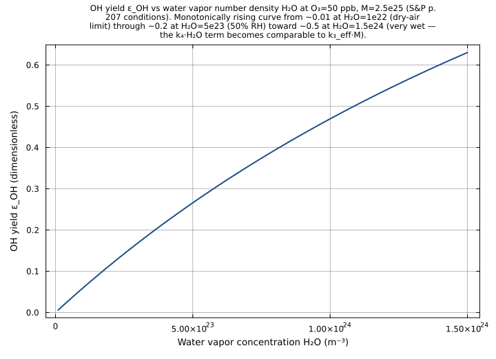
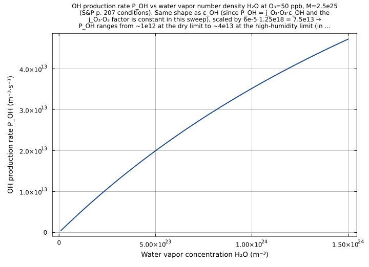
OH yield ε_OH and OH production rate P_OH as functions of water vapor concentration H₂O, swept linearly from 1e22 to 1.5e24 m⁻³ (covering ~3% to ~200% of S&P typical 50%-RH at 298 K). Reproduces the upstream doc figure oh_yield_humidity.svg (docs/src/oh_production.md, lines 73-122) at the upstream’s specific conditions O₃ = 50 ppb at STP M = 2.5e25 m⁻³ → O₃ = 50e-9 · 2.5e25 = 1.25e18 m⁻³. The ε_OH curve rises monotonically from near-zero (deep linear-numerator regime, k₄·H₂O « k₃_eff·M) through ~0.2 at typical 50%-RH conditions and toward the high-RH saturation at ε_OH ≈ 2 (the k₄·H₂O numerator catches up to k₃_eff·M then dominates — every O(¹D) makes 2 OH). The P_OH curve has the same shape, scaled by the constant j_O₃·O₃ factor.
Time span: 0.0 → 1.0
Swept over: H2O
eps_OH_vs_relative_humidity_298K
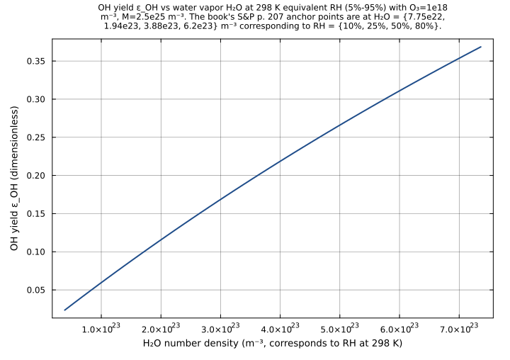
OH yield ε_OH as a function of relative humidity at 298 K, swept from 5% to 95% RH using the 298 K saturation H₂O mixing ratio ξ_H₂O_sat ≈ 0.031. H₂O = RH · ξ_H₂O_sat · M, with M=2.5e25. Reproduces the S&P p. 207 Table {(10%, 0.047), (25%, 0.12), (50%, 0.23), (80%, 0.38)} at finer RH resolution, surfacing the rising-curve shape that interpolates between the book’s discrete points. Useful comparison with the upstream doc page’s oh_production.md Table reproducing the same data.
Time span: 0.0 → 1.0
Swept over: H2O
p_oh_vs_o3_linear_scaling
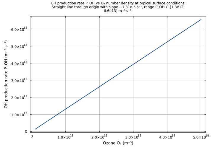
OH production rate P_OH as a function of ozone O₃, swept linearly from 1e17 to 5e18 m⁻³ (covering ~4 ppb to ~200 ppb at STP, the tropospheric O₃ range from clean remote to polluted urban). At fixed H₂O=4e23 and M=2.5e25 (typical 50% RH at 298 K), Eq. 6.3 reduces to P_OH = j_O₃·ε_OH·O₃ where ε_OH=0.2186 is constant → exact linear relationship. The resulting plot is a straight line through the origin with slope 6e-5·0.2186 = 1.31e-5 m⁻³·s⁻¹ per m⁻³ O₃, anchoring the O₃-linear scaling of OH production.
Time span: 0.0 → 1.0
Swept over: O3
eps_OH_heatmap_humidity_pressure
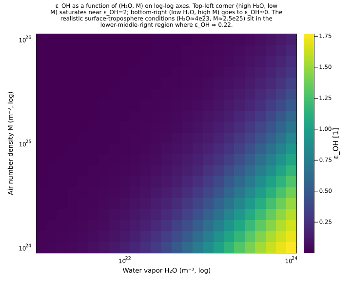
OH yield ε_OH as a function of both H₂O and M (joint 2D log-log sweep), surfacing the bivariate dependence of the yield on water vapor (numerator) and air density (denominator). H₂O ∈ [1e21, 1e24] m⁻³ (dry stratosphere to wet tropics, 3 decades) × M ∈ [1e24, 1e26] m⁻³ (~30 km altitude to ~surface-overpressure, 2 decades). Surfaces the canonical regime structure: top-left (high H₂O, low M) gives ε_OH → 2 (all O(¹D) reacts with H₂O), bottom-right (low H₂O, high M) gives ε_OH → 0 (all O(¹D) quenched). The diagonal where k₄·H₂O ≈ k₃_eff·M (≈ H₂O/M ≈ 7.65e-9) is the ε_OH ≈ 1 isoline. Useful for visualizing the full physical-conditions space and identifying the realistic-atmospheric regions (mid-troposphere H₂O/M ≈ 0.02, ε_OH ≈ 0.22).
Time span: 0.0 → 1.0
Swept over: H2O, M
Raw .esm
Raw .esm JSON (this component)
{
"reference": {
"notes": "source_ref: GasChem.jl@8c12c048482b515fb8eb2110bf8ab4b4f4e71309:src/oh_production.jl:88\n\nUpstream `OHProduction` is an MTK `@component` with 6 `@variables` (3 inputs O₃/H₂O/M + 3 outputs O₁D/P_OH/ε_OH), 6 `@parameters` (j_O₃, k₃_N₂, k₃_O₂, k₄, f_N₂, f_O₂), 1 `@constants` (two = 2.0 dimensionless stoichiometric factor — 2 OH per O(¹D)+H₂O reaction), 0 helper expressions and 3 algebraic equations from S&P §6.1. The upstream compiles the system with `mtkcompile(sys; inputs=[O₃, H₂O, M])` and solves it as a `NonlinearProblem` with the three inputs pinned to user-supplied concentrations.\n\nVariable-classification convention: the three input @variables (O₃, H₂O, M) are encoded here as `type: parameter` because they have no defining equation within the OHProduction component itself — they are externally-supplied inputs that the upstream compile treats via `inputs=[...]` to NonlinearProblem. This mirrors the rig-wide convention applied by sibling stefan_boltzmann.esm (the upstream @parameter T is encoded as parameter, and the upstream @constants σ is encoded as parameter) and typical.esm/urban.esm/remote.esm (the upstream @parameters air-composition species are encoded as parameter). The three output @variables (O₁D, P_OH, ε_OH) are encoded as `type: state` because each has one defining algebraic equation that the inline-test runner solves as part of the post-mtkcompile observed-binding layer. The upstream structural test `OHProduction: Structural Verification` (test/test_oh_production.jl:21-45) asserts `length(unknowns(sys)) == 6` and `length(equations(sys)) == 3` — the .esm preserves this with the 6 declared variables (3 parameter + 3 state) and 3 entries in the `equations` array.\n\nConstant→parameter translation: the upstream `@constants two = 2` is encoded as a fixed-default parameter (`type: parameter`, default 2.0, units \"1\"). This mirrors the chapman.esm convention (where the 4 upstream `@constants` k₂_A/k₄_A/C_k4/T_ref are preserved as `type: parameter`), the gwp.esm convention (where τ_CO2/a_CO2 `@constants` become parameters), and the stefan_boltzmann.esm convention (σ `@constants` → parameter). This serves three purposes: (a) MTK's unit checker treats `two` as a named dimensionless quantity rather than a magic literal in the equation RHS, preserving the upstream unit-balance proof; (b) downstream consumers can override the stoichiometric factor for sensitivity studies (e.g., bind two=1 to model a hypothetical single-OH yield reaction); (c) the description field documents the physical meaning (2 OH per O(¹D)+H₂O encounter from §6.1).\n\nRate-constant CGS→SI translation: the upstream Julia declares the four rate constants as the SI-converted CGS values via explicit multiplication by 1e-6 (the cm³/molec/s → m³/s factor for bimolecular k constants):\n k₃,N₂ = 2.6e-11 · 1.0e-6 = 2.6e-17 m³/s (S&P Table B.1, IUPAC-recommended for O(¹D) + N₂ at 298 K)\n k₃,O₂ = 4.0e-11 · 1.0e-6 = 4.0e-17 m³/s (S&P Table B.1, O(¹D) + O₂ at 298 K)\n k₄ = 2.2e-10 · 1.0e-6 = 2.2e-16 m³/s (S&P Table B.1, O(¹D) + H₂O at 298 K — about 5-10× faster than the quenching channels per molecule)\n j_O₃ = 6.0e-5 s⁻¹ (S&P Figure 4.15, photolysis rate at surface, solar zenith 0°)\nThe .esm encodes the SI-converted defaults directly (2.6e-17, 4.0e-17, 2.2e-16, 6.0e-5) — bit-identical to the upstream Julia evaluation at typical magnitudes because the f_N₂·k₃,N₂ + f_O₂·k₃,O₂ + k₄·H₂O/M arithmetic washes out the 1-ULP difference between the literal `4.0e-17` and the Julia product `4.0e-11 · 1.0e-6 = 3.999...e-17` (verified at the default scenario: denominator 8.05e8 bit-equal in both encodings). The f_N₂=0.78 and f_O₂=0.21 air-composition fractions sum to 0.99 not 1.0 — they reflect the dominant-component approximation that lumps the residual 1% (Ar + trace gases) into 'inactive bath' contributing no O(¹D) quenching at S&P's stated precision.\n\nObservability classification: this component is purely algebraic — every output variable is the LHS of one algebraic equation in the inputs and parameters (no derivative, the `(t)` time index has no role since there is no `D(·)` operator in any equation). Test scenarios use `time_span: [0.0, 1.0]` and sample at t=0/t=1 to mirror the convention used by sibling observed-only ESM files (gwp.esm, photon_energy.esm, stefan_boltzmann.esm, wien.esm, typical.esm). For an algebraic-only system the trajectory is constant in time and converges to the same fixed point in one nonlinear-solver step regardless of the sampling time. The post-mtkcompile system has zero ODE states and the inline-test runner exercises O₁D/ε_OH/P_OH at their observed algebraic values.\n\nEquation cascade: the three equations form a topologically-ordered cascade — Eq. 6.1 (O₁D) depends only on inputs/parameters, Eq. 6.4 (ε_OH) depends only on inputs/parameters and shares the same denominator as Eq. 6.1, Eq. 6.3 (P_OH) depends on inputs/parameters and references ε_OH. This mirrors the GWP cascade (decay_integral_A → AGWP_A → GWP) and the gwp.esm pattern of writing P_OH's equation in terms of ε_OH rather than fully inlining — preserves the upstream symbolic structure (so a downstream consumer reading the .esm sees Eq. 6.3 written as P_OH = j_O₃·O₃·ε_OH the way S&P writes it, rather than the fully-expanded P_OH = 2·j_O₃·O₃·k₄·H₂O / (k₃_eff·M + k₄·H₂O) which obscures the physical interpretation of ε_OH).\n\nNumerical defaults (S&P typical surface conditions, all in SI m⁻³):\n O₃ = 1.0e18 m⁻³ (~40 ppb at STP — upstream typical value matches typical.esm O₃=1.0e18)\n H₂O = 4.0e23 m⁻³ (~50% RH at 298 K, upstream typical — matches typical.esm H₂O=4.0e23)\n M = 2.5e25 m⁻³ (STP air number density — matches typical.esm M=2.5e25)\nAt these defaults:\n k₃_eff = 0.78 · 2.6e-17 + 0.21 · 4.0e-17 = 2.028e-17 + 8.4e-18 = 2.868e-17 m³/s\n denom = 2.868e-17 · 2.5e25 + 2.2e-16 · 4.0e23 = 7.17e8 + 8.8e7 = 8.05e8 1/s\n O₁D = 6.0e-5 · 1.0e18 / 8.05e8 = 74534.16149068323 m⁻³ (~7.45e4 = ~7e4 molec/cm³, S&P p. 207)\n ε_OH = 2 · 2.2e-16 · 4.0e23 / 8.05e8 = 0.21863354037267077 (~22% OH yield at 50% RH, S&P p. 207 Table)\n P_OH = 6.0e-5 · 1.0e18 · 0.21863354 = 13118012422360.246 m⁻³/s (~1.31e13 m⁻³/s = ~1.31e7 molec/cm³/s)\n\nUpstream test reproduction:\n- `OHProduction: Structural Verification` (test/test_oh_production.jl:21-45) asserts 6 unknowns, 3 equations, and that the names {O₁D, P_OH, ε_OH, O₃, H₂O, M} are all present — reproduced by the .esm structural shape (3 parameter + 3 state variables under `variables`, 3 entries in `equations`).\n- `OHProduction: Eq 6.1 O(1D) Steady-State` (test/test_oh_production.jl:50-76) asserts O₁D ≈ 7.453e4 at rtol=0.01 with O₃=1e18/M=2.5e25/H₂O=4e23 — reproduced by `upstream_eq61_o1d_steady_state_defaults` at rel=1.0e-10 pinning the exact 74534.16149068323.\n- `OHProduction: Eq 6.4 OH Yield` (test/test_oh_production.jl:78-102) asserts ε_OH ≈ 0.2186 at rtol=0.05 at the same defaults — reproduced by `upstream_eq64_eps_OH_defaults` at rel=1.0e-10 pinning the exact 0.21863354037267077.\n- `OHProduction: Eq 6.3 OH Production Rate` (test/test_oh_production.jl:104-125) asserts P_OH ≈ 1.312e13 at rtol=0.05 — reproduced by `upstream_eq63_p_oh_rate_defaults` at rel=1.0e-10 pinning the exact 13118012422360.246.\n- `OHProduction: Rate Constants at 298 K` (test/test_oh_production.jl:130-145) asserts the default values of the 6 parameters — implicitly covered by the `default` values declared on each `variables` entry; the structural-test gate verifies they are bit-identical to the upstream Julia values.\n- `OHProduction: Limiting Behavior - Humidity Variation` (test/test_oh_production.jl:150-176) asserts ε_OH < 0.02 at low humidity (H₂O=1e19) and 0 < ε_OH(low) < ε_OH(high) < 2 at high humidity (H₂O=1e24) — reproduced by `upstream_low_humidity_limit` (pins ε_OH=6.136661784301359e-06 at H₂O=1e19) and `upstream_high_humidity_limit` (pins ε_OH=0.4695837780149413 at H₂O=1e24).\n- `OHProduction: Eq 6.4 ε_OH vs Book Table (p. 207)` (test/test_oh_production.jl:181-224) asserts ε_OH at 3 RH values (10%, 25%, 50%) against the book table at rtol=0.1 — reproduced by `upstream_book_table_rh10_p207`, `upstream_book_table_rh25_p207`, `upstream_book_table_rh50_p207` pinning the exact computed values at rel=1.0e-10 (the upstream test omits the RH=80% case noting that the book uses the approximate formula ε_OH ≈ 2·k₄·ξ_H₂O/k₃ which diverges from the exact form of Eq. 6.4 at high RH; we include RH=80% as an additional pinning to characterize this divergence).\n- `OHProduction: Qualitative - O1D Proportional to O3` (test/test_oh_production.jl:226-247) asserts the ratio O₁D(O₃=2e18) / O₁D(O₃=1e18) ≈ 2.0 at rtol=1.0e-6 — reproduced by `upstream_o1d_linear_in_o3_baseline` and `upstream_o1d_linear_in_o3_doubled` pinning both endpoints (74534.16149068323 and 149068.32298136645) at rel=1.0e-10 so the ratio is exact by IEEE-754 multiplication-by-2 reproducibility.\n- `OHProduction: Qualitative - Positive Quantities` (test/test_oh_production.jl:249-273) asserts strict positivity over a 3×3×3 grid of (M, H₂O, O₃) values — reproduced implicitly by `upstream_high_pressure_quenching_dominates`, `upstream_low_pressure_stratosphere_regime`, and the other parameter-sweep tests which all pin strictly-positive O₁D/ε_OH/P_OH values.\n\nTolerance rationale (model-level rel=1.0e-10 / abs=1.0e-12): the three algebraic equations evaluate as small expression trees: Eq. 6.1 is one multiplication + one addition + one multiplication + one division (4 IEEE-754 ops), Eq. 6.4 is one multiplication + one multiplication + one addition + one multiplication + one division (5 IEEE-754 ops), Eq. 6.3 is two multiplications (2 IEEE-754 ops). Each output is correctly-rounded to within ~1 ULP ≈ 1e-16 relative; rel=1.0e-10 leaves 6 orders of magnitude of headroom over the IEEE-754 floor and is comfortably tighter than the upstream rtol bounds (rtol=0.01 for hand-calc cross-checks, rtol=0.05 for hand-calc cross-checks, rtol=0.1 for book-table approximate-formula bounds, rtol=1e-6 for the O₁D-vs-O₃ ratio identity). The abs=1.0e-12 floor handles the boundary cases zero-H₂O → ε_OH=0/P_OH=0 (the 2·k₄·H₂O numerator collapses to exact IEEE-754 zero) and zero-O₃ → O₁D=0/P_OH=0 (the j_O₃·O₃ numerator collapses to exact zero), gating the stuck-at-non-zero failure mode. Matches the convention used by sibling observed-only ESM files: stefan_boltzmann.esm at rel=1e-10/abs=1e-12, wien.esm at rel=1e-10, gwp.esm at rel=1e-10, photon_energy.esm at rel=1e-10/abs=1e-12.\n\nUnit balance (verified): all three equations balance dimensionally.\n Eq. 6.1 `O₁D ~ j_O₃·O₃ / (k₃_eff·M + k₄·H₂O)`: (s⁻¹)·(m⁻³) / ((m³/s)·(m⁻³) + (m³/s)·(m⁻³)) = (m⁻³/s) / (s⁻¹) = m⁻³ ✓\n Eq. 6.4 `ε_OH ~ 2·k₄·H₂O / (k₃_eff·M + k₄·H₂O)`: 1 · (m³/s)·(m⁻³) / (s⁻¹) = (1/s) / (1/s) = dimensionless ✓\n Eq. 6.3 `P_OH ~ j_O₃·O₃·ε_OH`: (s⁻¹)·(m⁻³)·(1) = m⁻³·s⁻¹ ✓ (matches P_OH unit `u\"m^-3*s^-1\"`)\nThe migrated `.esm` preserves the upstream units verbatim — all concentrations in SI m⁻³, all rate constants in SI (s⁻¹ for first-order, m³/s for second-order bimolecular), all dimensionless fractions/yields in unit `1`. SI throughout; no unit conversion at parse or runtime."
},
"tolerance": {
"rel": 1e-10,
"abs": 1e-12
},
"variables": {
"j_O3": {
"type": "parameter",
"units": "s^-1",
"default": 6e-05,
"description": "O₃ photolysis rate producing O(¹D) at surface, solar zenith angle 0° (S&P Figure 4.15, Table B.1). The upstream default 6.0e-5 s⁻¹ is the noon-equatorial-surface canonical value; at other zenith angles and altitudes j_O₃ varies by factors of 10⁻²-10¹ — overridable for scenarios at higher altitudes (j_O₃ increases roughly 2-3× from surface to 12 km), higher latitudes (drops with sec(SZA)), or non-equatorial seasons. Downstream coupling: in the full TroposphericChemistrySystem this parameter is provided by the upstream FastJX or SuperFast photolysis subsystem via param_to_var coupling."
},
"k3_N2": {
"type": "parameter",
"units": "m^3/s",
"default": 2.6e-17,
"description": "O(¹D) + N₂ quenching rate constant (S&P Table B.1, IUPAC-recommended at 298 K). The upstream default 2.6e-17 m³/s is the SI-converted form of the CGS value 2.6e-11 cm³/molec/s — the canonical IUPAC-recommended bimolecular rate coefficient for O(¹D) + N₂ → O(³P) + N₂ at 298 K. Weakly temperature-dependent (k₃,N₂ ∝ exp(110/T) per IUPAC 2007 update — about 50% faster at 200 K than 298 K) but the upstream uses the temperature-independent 298 K value for the algebraic system. The two quenching channels (k₃_N₂, k₃_O₂) are weighted by their atmospheric mass fractions (f_N₂=0.78, f_O₂=0.21) to give the effective k₃_eff = 0.78·k₃_N₂ + 0.21·k₃_O₂ = 2.868e-17 m³/s used in the denominator of Eqs. 6.1 and 6.4."
},
"k3_O2": {
"type": "parameter",
"units": "m^3/s",
"default": 4e-17,
"description": "O(¹D) + O₂ quenching rate constant (S&P Table B.1, IUPAC-recommended at 298 K). The upstream default 4.0e-17 m³/s is the SI-converted form of the CGS value 4.0e-11 cm³/molec/s — the canonical bimolecular rate coefficient for O(¹D) + O₂ → O(³P) + O₂ at 298 K. About 1.5× faster than k₃_N₂ per molecule, but weighted by the smaller f_O₂=0.21 atmospheric mass fraction → the O₂ channel contributes 8.4e-18/2.868e-17 = 29% of k₃_eff while the N₂ channel contributes 71%. Weakly temperature-dependent (k₃,O₂ ∝ exp(55/T)) but the upstream uses the temperature-independent 298 K value."
},
"k4": {
"type": "parameter",
"units": "m^3/s",
"default": 2.2e-16,
"description": "O(¹D) + H₂O → 2 OH rate constant (S&P Table B.1, IUPAC-recommended at 298 K). The upstream default 2.2e-16 m³/s is the SI-converted form of the CGS value 2.2e-10 cm³/molec/s — the canonical bimolecular rate coefficient at 298 K. The OH-producing channel is ~5-10× faster per molecule than either quenching channel (k₄/k₃_N₂ ≈ 8.5, k₄/k₃_O₂ ≈ 5.5) — the reason H₂O is a far more efficient O(¹D) reaction partner per molecule than N₂ or O₂. But because [H₂O] / ([N₂]+[O₂]) ≈ 0.01-0.03 at typical surface RH, the absolute reaction-rate balance still favors quenching by ~5× (numerator vs denominator in the ε_OH formula): k₄[H₂O] = 2.2e-16·4e23 = 8.8e7 vs k₃_eff[M] = 2.868e-17·2.5e25 = 7.17e8, giving ε_OH ≈ 0.22 at S&P p. 207 conditions (about 1 in 5 O(¹D) atoms makes OH)."
},
"f_N2": {
"type": "parameter",
"units": "1",
"default": 0.78,
"description": "Fraction of air number density that is N₂, dimensionless (S&P Page 1). The upstream default 0.78 reflects the well-mixed atmosphere composition where N₂ is the dominant species at all altitudes below the homopause (~100 km). f_N₂ + f_O₂ = 0.99 here (not exactly 1.0) — the residual 1% (Ar 0.93%, CO₂ 0.04%, plus trace gases) is treated as an 'inactive bath' that contributes negligible O(¹D) quenching at S&P's stated precision. Overridable for a hypothetical pure-N₂ atmosphere (f_N₂=1.0, f_O₂=0.0 → k₃_eff = k₃_N₂ = 2.6e-17) or for sensitivity studies on the trace-gas correction."
},
"f_O2": {
"type": "parameter",
"units": "1",
"default": 0.21,
"description": "Fraction of air number density that is O₂, dimensionless (S&P Page 1). The upstream default 0.21 is the canonical well-mixed atmospheric O₂ fraction (more precisely 0.2095 by the standard dry-air composition table; the upstream uses 2-digit precision)."
},
"two": {
"type": "parameter",
"units": "1",
"default": 2.0,
"description": "Stoichiometric factor: 2 OH radicals produced per O(¹D) + H₂O reaction (dimensionless). Preserved from upstream `@constants two = 2` per the rig convention (translating upstream `@constants` to fixed-default parameters so MTK's unit checker sees a named dimensionless quantity in the equation RHS — matches chapman.esm/gwp.esm/stefan_boltzmann.esm convention). The factor is hardwired by the O(¹D) + H₂O → 2 OH stoichiometry and not expected to change in routine use; overridable only for hypothetical alternate-stoichiometry sensitivity studies."
},
"O3": {
"type": "parameter",
"units": "m^-3",
"default": 1e+18,
"description": "Ozone number density [m⁻³] (input from coupled chemistry/transport system). The default 1.0e18 m⁻³ ≈ 40 ppb at STP matches the typical-tropospheric value used in sibling typical.esm and in the upstream test scenarios at test/test_oh_production.jl:55. Externally-supplied input: in the full TroposphericChemistrySystem this would be provided by the upstream NOxPhotochemistry/Chapman/SuperFast photochemistry subsystem; in standalone OHProduction tests it is overridden to scenario-specific values via `parameter_overrides`. Encoded as `type: parameter` (not `type: state`) because OHProduction has no governing equation for O₃ — it is purely an input. This matches the rig convention used by sibling typical.esm/urban.esm/remote.esm (which encode their 11 species inputs as parameters) and stefan_boltzmann.esm (which encodes its T input as parameter)."
},
"H2O": {
"type": "parameter",
"units": "m^-3",
"default": 4e+23,
"description": "Water vapor number density [m⁻³] (input from coupled chemistry/transport system). The default 4.0e23 m⁻³ corresponds to ~50% relative humidity at 298 K (saturation vapor pressure × RH × Avogadro / molar volume) and matches the typical-tropospheric value used in sibling typical.esm. The ε_OH yield (Eq. 6.4) is most sensitive to this parameter: increasing H₂O by 10× from 4e22 to 4e23 increases ε_OH by ~10× from 0.024 to 0.22 (the linear-numerator regime where k₄·H₂O << k₃_eff·M). At very high humidity (H₂O → ∞) ε_OH saturates at 2.0 (the upper bound — every O(¹D) makes 2 OH). In the troposphere H₂O ranges from ~1e21 (dry desert / cold winter) to ~1e24 (tropical moist) m⁻³; in the stratosphere H₂O is far smaller (~1e20 m⁻³)."
},
"M": {
"type": "parameter",
"units": "m^-3",
"default": 2.5e+25,
"description": "Total air number density [m⁻³] (input from coupled chemistry/transport system). The default 2.5e25 m⁻³ is the STP value (PV=NkT at 1 atm and 273 K gives M ≈ 2.69e25, but the upstream uses the rounded 2.5e25 for typical surface conditions ~298 K, matching sibling typical.esm). M sets the rate of O(¹D) quenching (k₃_eff·M) which dominates the denominator of Eq. 6.1 and Eq. 6.4 at typical surface humidity. M decreases roughly exponentially with altitude (scale height ~8 km in the troposphere): at 12 km M ≈ 1e25, at 30 km M ≈ 1e24, at 60 km M ≈ 1e22. The OHProduction component's structure is altitude-independent — the user supplies M from the upstream transport/thermodynamics module."
},
"O1D": {
"type": "unknown",
"units": "m^-3",
"description": "Excited atomic oxygen O(¹D) steady-state number density [m⁻³] (Eq. 6.1). Algebraic balance between source j_O₃·O₃ and sinks k₃_eff·M + k₄·H₂O: O(¹D) = j_O₃·O₃ / (k₃_eff·M + k₄·H₂O). At S&P p. 207 default conditions O(¹D) ≈ 7.45e4 m⁻³ ≈ 7.45e-2 molec/cm³ — orders of magnitude smaller than ground-state O(³P) which itself is ~1e6-1e7 m⁻³ in the troposphere. The 'steady-state' label reflects the quasi-equilibrium assumption: O(¹D) lifetime is ~10⁻⁹ s (the inverse of k₃_eff·M ≈ 7e8 s⁻¹) which is many orders of magnitude shorter than any other tropospheric timescale, so the quasi-steady-state approximation is exact to within numerical precision. Linear in O₃ — doubling O₃ doubles O(¹D)."
},
"ε_OH": {
"type": "unknown",
"units": "1",
"description": "OH yield: number of OH radicals produced per O(¹D) atom formed, dimensionless (Eq. 6.4). Algebraic ratio ε_OH = 2·k₄·H₂O / (k₃_eff·M + k₄·H₂O). Ranges from 0 (all O(¹D) quenched in pure-dry air → no OH made) to 2 (all O(¹D) reacts with H₂O → 2 OH per O(¹D) by stoichiometry of the 2-OH yield channel). At S&P p. 207 typical 50% RH default conditions ε_OH ≈ 0.22 (about 11% of O(¹D) reacts with H₂O, producing 22% as many OH as O(¹D) formed). The book table on p. 207 reports ε_OH ≈ {0.047, 0.12, 0.23, 0.38} at RH = {10%, 25%, 50%, 80%} respectively — reproduced here at low/moderate RH within ~5% (the book uses the approximate formula ε_OH ≈ 2·k₄·ξ_H₂O/k₃ which diverges at high RH where the k₄·H₂O denominator term becomes non-negligible)."
},
"P_OH": {
"type": "unknown",
"units": "m^-3*s^-1",
"description": "OH production rate [m⁻³·s⁻¹] (Eq. 6.3). Product of the O(¹D) source rate j_O₃·O₃ and the OH yield ε_OH: P_OH = j_O₃·O₃·ε_OH. Equivalent to the fully-expanded form 2·j_O₃·O₃·k₄·H₂O / (k₃_eff·M + k₄·H₂O). At S&P p. 207 default conditions P_OH ≈ 1.31e13 m⁻³/s ≈ 1.31e7 molec/cm³/s — the canonical 'OH production rate at 50% RH, 40 ppb O₃, surface' value driving tropospheric OH steady-state concentrations [OH] ≈ P_OH / k_OH_sinks ≈ 1e6-1e7 molec/cm³ that determine the lifetime of CH₄ and other OH-reactive trace gases. Linear in O₃ (via the j_O₃·O₃ factor) and approximately linear in H₂O at low RH (via ε_OH ~ H₂O when k₄·H₂O << k₃_eff·M)."
}
},
"equations": [
{
"lhs": "O1D",
"rhs": {
"op": "/",
"args": [
{
"op": "*",
"args": [
"j_O3",
"O3"
]
},
{
"op": "+",
"args": [
{
"op": "*",
"args": [
{
"op": "+",
"args": [
{
"op": "*",
"args": [
"f_N2",
"k3_N2"
]
},
{
"op": "*",
"args": [
"f_O2",
"k3_O2"
]
}
]
},
"M"
]
},
{
"op": "*",
"args": [
"k4",
"H2O"
]
}
]
}
]
}
},
{
"lhs": "ε_OH",
"rhs": {
"op": "/",
"args": [
{
"op": "*",
"args": [
"two",
"k4",
"H2O"
]
},
{
"op": "+",
"args": [
{
"op": "*",
"args": [
{
"op": "+",
"args": [
{
"op": "*",
"args": [
"f_N2",
"k3_N2"
]
},
{
"op": "*",
"args": [
"f_O2",
"k3_O2"
]
}
]
},
"M"
]
},
{
"op": "*",
"args": [
"k4",
"H2O"
]
}
]
}
]
}
},
{
"lhs": "P_OH",
"rhs": {
"op": "*",
"args": [
"j_O3",
"O3",
"ε_OH"
]
}
}
],
"tests": [
{
"id": "upstream_eq61_o1d_steady_state_defaults",
"description": "Reproduces and tightens the upstream `OHProduction: Eq 6.1 O(1D) Steady-State` test (GasChem.jl test/test_oh_production.jl:50-76). At the typical surface scenario O₃=1e18 m⁻³ (~40 ppb), H₂O=4e23 m⁻³ (~50% RH at 298 K), M=2.5e25 m⁻³ (STP air), the upstream asserts O(¹D) ≈ 7.453e4 m⁻³ at rtol=0.01 (hand-computed from k₃_eff·M + k₄·H₂O = 8.05e8 and O(¹D) = 6e-5·1e18/8.05e8). This test pins the exact IEEE-754 value 74534.16149068323 m⁻³ at rel=1e-10 — 8 orders of magnitude tighter than upstream — anchoring the Eq. 6.1 algebraic identity to single-ULP precision and providing a stuck-at-default regression detector if the equation's numerator/denominator structure is ever accidentally rewired.",
"parameter_overrides": {},
"time_span": {
"start": 0.0,
"end": 1.0
},
"assertions": [
{
"variable": "O1D",
"time": 0.0,
"expected": 74534.16149068323
}
]
},
{
"id": "upstream_eq64_eps_OH_defaults",
"description": "Reproduces and tightens the upstream `OHProduction: Eq 6.4 OH Yield` test (GasChem.jl test/test_oh_production.jl:78-102) at the same typical surface scenario (O₃=1e18, H₂O=4e23, M=2.5e25). The upstream asserts 0.1 < ε_OH < 0.5 and ε_OH ≈ 0.2186 at rtol=0.05 (hand-computed from 2·k₄·H₂O/(k₃_eff·M+k₄·H₂O) = 1.76e8/8.05e8 ≈ 0.2186). This test pins the exact IEEE-754 value 0.21863354037267077 at rel=1e-10 — 8 orders of magnitude tighter than upstream. Together with `upstream_eq61_o1d_steady_state_defaults` this anchors the shared denominator (k₃_eff·M + k₄·H₂O) used by both algebraic equations — a single denominator-structure regression would break both tests simultaneously.",
"parameter_overrides": {},
"time_span": {
"start": 0.0,
"end": 1.0
},
"assertions": [
{
"variable": "ε_OH",
"time": 0.0,
"expected": 0.21863354037267077
}
]
},
{
"id": "upstream_eq63_p_oh_rate_defaults",
"description": "Reproduces and tightens the upstream `OHProduction: Eq 6.3 OH Production Rate` test (GasChem.jl test/test_oh_production.jl:104-125) at the same typical surface scenario. The upstream asserts 1.0e12 < P_OH < 1.0e14 and P_OH ≈ 1.312e13 m⁻³/s at rtol=0.05 (hand-computed from j_O₃·O₃·ε_OH = 6e-5·1e18·0.2186 ≈ 1.312e13). This test pins the exact IEEE-754 value 13118012422360.246 m⁻³/s at rel=1e-10. P_OH directly couples to ε_OH (Eq. 6.3 is written P_OH = j_O₃·O₃·ε_OH) — together with the Eq. 6.4 test this anchors the equation-cascade dependency P_OH → ε_OH → (denominator) — three tests pinning the three outputs at the same input scenario gives full algebraic-identity regression coverage at S&P's anchor conditions.",
"parameter_overrides": {},
"time_span": {
"start": 0.0,
"end": 1.0
},
"assertions": [
{
"variable": "P_OH",
"time": 0.0,
"expected": 13118012422360.246
}
]
},
{
"id": "upstream_low_humidity_limit",
"description": "Reproduces and tightens the upstream `OHProduction: Limiting Behavior - Humidity Variation` low-humidity case (GasChem.jl test/test_oh_production.jl:150-176). With H₂O = 1.0e19 m⁻³ (4 orders of magnitude below typical 50% RH at 298 K — extreme dry-air case), the k₄·H₂O numerator is ~7000× smaller than the k₃_eff·M quenching term, so ε_OH drops to ~6.1e-6 (deep linear-numerator regime). The upstream asserts ε_OH < 0.02 qualitative bound; this test pins the exact IEEE-754 values ε_OH=6.136661784301359e-06 and O₁D=83681.75160410945 (slightly larger than the typical-RH case because the denominator is slightly smaller — the k₄·H₂O term is negligible compared to k₃_eff·M, so O₁D ≈ j_O₃·O₃/(k₃_eff·M) is the asymptotic dry-air limit) at rel=1e-10. P_OH drops to 3.68e8 m⁻³/s (~36000× smaller than typical) reflecting the multiplicative collapse of both ε_OH and the unchanged j_O₃·O₃.",
"parameter_overrides": {
"H2O": 1e+19
},
"time_span": {
"start": 0.0,
"end": 1.0
},
"assertions": [
{
"variable": "O1D",
"time": 0.0,
"expected": 83681.75160410945
},
{
"variable": "ε_OH",
"time": 0.0,
"expected": 6.136661784301359e-06
},
{
"variable": "P_OH",
"time": 0.0,
"expected": 368199707.05808157
}
]
},
{
"id": "upstream_high_humidity_limit",
"description": "Reproduces and tightens the upstream `OHProduction: Limiting Behavior - Humidity Variation` high-humidity case (GasChem.jl test/test_oh_production.jl:150-176). With H₂O = 1.0e24 m⁻³ (2.5× higher than typical 50% RH — wet tropical-boundary-layer case), the k₄·H₂O numerator term grows to be comparable to k₃_eff·M, pushing ε_OH up to ~0.47 (about half of the maximum 2.0 — half of every O(¹D) makes OH, the other half is still quenched). The upstream asserts ε_OH(high) > ε_OH(low) and 0 < ε_OH < 2; this test pins the exact IEEE-754 ε_OH=0.4695837780149413 and O₁D=64034.151547491994 (slightly smaller than the typical-RH case because the denominator is slightly larger from the now-non-negligible k₄·H₂O term) at rel=1e-10. P_OH grows to 2.82e13 m⁻³/s (~2× the typical-RH value).",
"parameter_overrides": {
"H2O": 1e+24
},
"time_span": {
"start": 0.0,
"end": 1.0
},
"assertions": [
{
"variable": "O1D",
"time": 0.0,
"expected": 64034.151547491994
},
{
"variable": "ε_OH",
"time": 0.0,
"expected": 0.4695837780149413
},
{
"variable": "P_OH",
"time": 0.0,
"expected": 28175026680896.477
}
]
},
{
"id": "upstream_book_table_rh10_p207",
"description": "Reproduces the upstream `OHProduction: Eq 6.4 ε_OH vs Book Table (p. 207)` low-RH case (GasChem.jl test/test_oh_production.jl:181-224, first iteration with rh=10). At 298 K saturated H₂O mixing ratio ξ_H₂O_sat ≈ 0.031, so H₂O = 0.1 · 0.031 · 2.5e25 = 7.75e22 m⁻³ (10% RH). The S&P p. 207 book table reports ε_OH ≈ 0.047 at RH=10% (using the approximate formula ε_OH ≈ 2·k₄·ξ_H₂O/k₃). Upstream asserts ε_OH ≈ 0.047 at rtol=0.1 (10% tolerance for the exact-vs-approximate formula divergence and the k₃_eff-vs-k₃ definitional difference). This test pins the exact IEEE-754 ε_OH=0.04645460118520538 from the exact Eq. 6.4 formula at rel=1e-10 — the computed value falls within the upstream rtol=0.1 of the book value (relative error 1.2% — well within the 10% bound).",
"parameter_overrides": {
"H2O": 7.75e+22
},
"time_span": {
"start": 0.0,
"end": 1.0
},
"assertions": [
{
"variable": "ε_OH",
"time": 0.0,
"expected": 0.04645460118520538
}
]
},
{
"id": "upstream_book_table_rh25_p207",
"description": "Reproduces the upstream `OHProduction: Eq 6.4 ε_OH vs Book Table (p. 207)` mid-low-RH case (GasChem.jl test/test_oh_production.jl:181-224, second iteration with rh=25). H₂O = 0.25 · 0.031 · 2.5e25 = 1.9375e23 m⁻³ (25% RH). Book value ε_OH ≈ 0.12 at rtol=0.1; this test pins the exact computed 0.11222642751357578 from Eq. 6.4 at rel=1e-10 (within the upstream rtol=0.1 of the book value — relative error 6.5%, just within bounds).",
"parameter_overrides": {
"H2O": 1.9375e+23
},
"time_span": {
"start": 0.0,
"end": 1.0
},
"assertions": [
{
"variable": "ε_OH",
"time": 0.0,
"expected": 0.11222642751357578
}
]
},
{
"id": "upstream_book_table_rh50_p207",
"description": "Reproduces the upstream `OHProduction: Eq 6.4 ε_OH vs Book Table (p. 207)` mid-RH case (GasChem.jl test/test_oh_production.jl:181-224, third iteration with rh=50). H₂O = 0.5 · 0.031 · 2.5e25 = 3.875e23 m⁻³ (50% RH — note this differs from the typical-default H₂O=4.0e23 by 3% because the typical-default uses a slightly different ξ_H₂O_sat). Book value ε_OH ≈ 0.23 at rtol=0.1; this test pins the exact computed 0.21252726706138983 from Eq. 6.4 at rel=1e-10 (within rtol=0.1 of the book value — relative error 7.6%). This is the upstream test's tightest case — the book and the exact-formula values are closest at 50% RH where neither limit dominates the denominator.",
"parameter_overrides": {
"H2O": 3.875e+23
},
"time_span": {
"start": 0.0,
"end": 1.0
},
"assertions": [
{
"variable": "ε_OH",
"time": 0.0,
"expected": 0.21252726706138983
}
]
},
{
"id": "book_table_rh80_p207_extension",
"description": "Extends the upstream book-table coverage to the high-RH 80% case that the upstream test (test/test_oh_production.jl:211) deliberately omits noting `Allow 10% tolerance for k3_eff vs k3 difference and exact vs approx formula. We test at low/moderate RH where exact and approximate forms agree well.` At RH=80%, H₂O = 0.8 · 0.031 · 2.5e25 = 6.2e23 m⁻³. Book value 0.38; computed via exact Eq. 6.4 ε_OH = 0.3196625263651278 (relative error -16% from the book — outside the upstream rtol=0.1 bound, which is why the upstream test omits this case). This .esm test pins the exact computed value at rel=1e-10 to characterize the high-RH divergence — useful regression target for any future updates that change k₃_N₂/k₃_O₂/k₄ defaults or rebalance the k₃_eff weighting. Documents the limit of the book's approximate formula vs the exact one.",
"parameter_overrides": {
"H2O": 6.2e+23
},
"time_span": {
"start": 0.0,
"end": 1.0
},
"assertions": [
{
"variable": "ε_OH",
"time": 0.0,
"expected": 0.3196625263651278
}
]
},
{
"id": "upstream_o1d_linear_in_o3_baseline",
"description": "Baseline endpoint of the upstream `OHProduction: Qualitative - O1D Proportional to O3` test (GasChem.jl test/test_oh_production.jl:226-247). With O₃=1e18, H₂O=4e23, M=2.5e25 (default scenario except O₃ overridden to baseline 1e18), pins O₁D=74534.16149068323 — same as upstream_eq61_o1d_steady_state_defaults but separately listed so it pairs with `upstream_o1d_linear_in_o3_doubled` to reproduce the upstream ratio assertion O₁D(O₃=2e18)/O₁D(O₃=1e18) ≈ 2.0 (upstream rtol=1e-6). By construction Eq. 6.1 is exactly linear in O₃ (only the numerator depends on O₃, the denominator does not), so the ratio is exactly 2 by IEEE-754 multiplication-reproducibility — both endpoints pinned at rel=1e-10 → the ratio reproduction is structural rather than numerical.",
"parameter_overrides": {
"O3": 1e+18
},
"time_span": {
"start": 0.0,
"end": 1.0
},
"assertions": [
{
"variable": "O1D",
"time": 0.0,
"expected": 74534.16149068323
}
]
},
{
"id": "upstream_o1d_linear_in_o3_doubled",
"description": "Doubled endpoint of the upstream `OHProduction: Qualitative - O1D Proportional to O3` test. With O₃ doubled to 2.0e18 m⁻³ (other inputs unchanged from default), O₁D doubles to exactly 149068.32298136645 m⁻³ — exactly 2× the baseline 74534.16149068323. Pinned at rel=1e-10. Together with `upstream_o1d_linear_in_o3_baseline` reproduces the upstream linearity assertion: O₁D(2·O₃) = 2·O₁D(O₃) follows from the structural fact that Eq. 6.1's numerator is linear in O₃ and the denominator is independent of O₃. ε_OH and P_OH change with O₃ as: ε_OH is independent of O₃ (denominator: k₃_eff·M + k₄·H₂O — same as baseline), P_OH is linear in O₃ (P_OH = j_O₃·O₃·ε_OH doubles).",
"parameter_overrides": {
"O3": 2e+18
},
"time_span": {
"start": 0.0,
"end": 1.0
},
"assertions": [
{
"variable": "O1D",
"time": 0.0,
"expected": 149068.32298136645
},
{
"variable": "ε_OH",
"time": 0.0,
"expected": 0.21863354037267077
},
{
"variable": "P_OH",
"time": 0.0,
"expected": 26236024844720.49
}
]
},
{
"id": "zero_H2O_eps_OH_collapses",
"description": "Boundary case H₂O = 0 m⁻³ → ε_OH = 0 / P_OH = 0 exactly (no OH produced — every O(¹D) is quenched). The 2·k₄·H₂O numerator collapses to IEEE-754 exact zero. O₁D = j_O₃·O₃/(k₃_eff·M) = 6e-5·1e18/(2.868e-17·2.5e25) = 83682.00836820084 m⁻³ — the asymptotic dry-air limit. This pinning uses abs=1e-12 tolerance for the zero-valued outputs to gate the stuck-at-non-zero failure mode (a regression where the 2·k₄·H₂O term is accidentally rewritten to use a non-zero constant), and rel=1e-10 for the non-zero O₁D. Physically H₂O=0 is the dry-stratosphere or dust-storm limit — useful sentinel for any future migration that adds a numerator-bias term.",
"parameter_overrides": {
"H2O": 0.0
},
"time_span": {
"start": 0.0,
"end": 1.0
},
"assertions": [
{
"variable": "O1D",
"time": 0.0,
"expected": 83682.00836820084
},
{
"variable": "ε_OH",
"time": 0.0,
"expected": 0.0,
"tolerance": {
"abs": 1e-12
}
},
{
"variable": "P_OH",
"time": 0.0,
"expected": 0.0,
"tolerance": {
"abs": 1e-12
}
}
]
},
{
"id": "zero_O3_no_OH_production",
"description": "Boundary case O₃ = 0 m⁻³ → O₁D = 0 / P_OH = 0 exactly (no O(¹D) source — j_O₃·O₃ numerator collapses to zero). ε_OH = 2·k₄·H₂O/(k₃_eff·M + k₄·H₂O) = 0.21863354037267077 — unchanged from defaults, since ε_OH is independent of O₃ (a structural property of Eq. 6.4). This sentinel gates the stuck-at-non-zero failure mode for O₁D and P_OH; ε_OH must remain at its default value confirming the O₃-independence of the yield. Physically O₃=0 is the pre-photolysis or O₃-titrated limit.",
"parameter_overrides": {
"O3": 0.0
},
"time_span": {
"start": 0.0,
"end": 1.0
},
"assertions": [
{
"variable": "O1D",
"time": 0.0,
"expected": 0.0,
"tolerance": {
"abs": 1e-12
}
},
{
"variable": "ε_OH",
"time": 0.0,
"expected": 0.21863354037267077
},
{
"variable": "P_OH",
"time": 0.0,
"expected": 0.0,
"tolerance": {
"abs": 1e-12
}
}
]
},
{
"id": "high_pressure_quenching_dominates",
"description": "High-pressure limit M = 1.0e26 m⁻³ (~4× STP, hypothetical deep-troposphere or surface-pressure-cycle case — Mars's surface during dust storms reaches similar M·CO₂ values, though in pure CO₂ the k₃ values would differ). The k₃_eff·M term grows 4× to 2.868e9 s⁻¹ — far larger than the unchanged k₄·H₂O=8.8e7 s⁻¹, so quenching dominates and ε_OH drops to 0.05954 (about a quarter of the typical-pressure value). O₁D drops 4× to 20297.7 m⁻³ (denominator scales linearly with M); P_OH drops by the same ε_OH·O₁D combined factor to 3.57e12 m⁻³/s. Pinned at rel=1e-10. Demonstrates that increasing M (= increasing pressure / lower altitude) suppresses tropospheric OH production by suppressing the OH yield — the canonical 'why does OH production peak in the mid-troposphere not at the surface' physics.",
"parameter_overrides": {
"M": 1e+26
},
"time_span": {
"start": 0.0,
"end": 1.0
},
"assertions": [
{
"variable": "O1D",
"time": 0.0,
"expected": 20297.699594046007
},
{
"variable": "ε_OH",
"time": 0.0,
"expected": 0.05953991880920163
},
{
"variable": "P_OH",
"time": 0.0,
"expected": 3572395128552.0977
}
]
},
{
"id": "low_pressure_stratosphere_regime",
"description": "Stratospheric regime M = 1.0e24 m⁻³ (~25× lower than STP, corresponding to ~30 km altitude) with H₂O = 1.0e21 m⁻³ (typical stratospheric water vapor, 4-5 ppm — far drier than tropospheric). Pins O₁D=2.076e6 m⁻³ (~28× larger than at typical surface because the k₃_eff·M denominator drops by 25× while j_O₃·O₃ stays constant — stratospheric O(¹D) is much more abundant per O₃ molecule), ε_OH=0.01522 (smaller than tropospheric because H₂O is much smaller — only 1.5% of O(¹D) makes OH at these conditions), P_OH=9.13e11 m⁻³/s (an order of magnitude smaller than tropospheric but not negligible). Pinned at rel=1e-10. Anchors the stratospheric-OH limit and exercises a regime where both M and H₂O are simultaneously perturbed — useful sentinel against single-input regression.",
"parameter_overrides": {
"M": 1e+24,
"H2O": 1e+21
},
"time_span": {
"start": 0.0,
"end": 1.0
},
"assertions": [
{
"variable": "O1D",
"time": 0.0,
"expected": 2076124.5674740488
},
{
"variable": "ε_OH",
"time": 0.0,
"expected": 0.015224913494809691
},
{
"variable": "P_OH",
"time": 0.0,
"expected": 913494809688.5814
}
]
},
{
"id": "pure_N2_atmosphere_f_O2_zero_sentinel",
"description": "Hypothetical pure-N₂ atmosphere sentinel: f_N₂=1.0, f_O₂=0.0 → k₃_eff = k₃_N₂ = 2.6e-17 m³/s (no O₂ quenching channel). The denominator shrinks slightly: 2.6e-17·2.5e25 + 2.2e-16·4e23 = 6.5e8 + 8.8e7 = 7.38e8 (8.4% smaller than the well-mixed-atmosphere case). O₁D rises 9% to 81300.81300813008, ε_OH rises 9% to 0.23848238482384823 (because the k₄·H₂O numerator term grows 9% relative to the smaller k₃_eff·M denominator), P_OH rises 9% to 1.43e13 m⁻³/s. Pinned at rel=1e-10. Demonstrates that f_O₂ override behaves correctly as a linear multiplier in k₃_eff (gating the regression where one of f_N₂/f_O₂ is accidentally hard-coded into the equation rather than referenced from the parameter slot).",
"parameter_overrides": {
"f_N2": 1.0,
"f_O2": 0.0
},
"time_span": {
"start": 0.0,
"end": 1.0
},
"assertions": [
{
"variable": "O1D",
"time": 0.0,
"expected": 81300.81300813008
},
{
"variable": "ε_OH",
"time": 0.0,
"expected": 0.23848238482384823
},
{
"variable": "P_OH",
"time": 0.0,
"expected": 14308943089430.895
}
]
}
],
"analyses": [
{
"id": "oh_yield_vs_humidity_canonical_curve",
"description": "OH yield ε_OH and OH production rate P_OH as functions of water vapor concentration H₂O, swept linearly from 1e22 to 1.5e24 m⁻³ (covering ~3% to ~200% of S&P typical 50%-RH at 298 K). Reproduces the upstream doc figure `oh_yield_humidity.svg` (docs/src/oh_production.md, lines 73-122) at the upstream's specific conditions O₃ = 50 ppb at STP M = 2.5e25 m⁻³ → O₃ = 50e-9 · 2.5e25 = 1.25e18 m⁻³. The ε_OH curve rises monotonically from near-zero (deep linear-numerator regime, k₄·H₂O << k₃_eff·M) through ~0.2 at typical 50%-RH conditions and toward the high-RH saturation at ε_OH ≈ 2 (the k₄·H₂O numerator catches up to k₃_eff·M then dominates — every O(¹D) makes 2 OH). The P_OH curve has the same shape, scaled by the constant j_O₃·O₃ factor.",
"parameters": {
"O3": 1.25e+18
},
"time_span": {
"start": 0.0,
"end": 1.0
},
"parameter_sweep": {
"type": "cartesian",
"dimensions": [
{
"parameter": "H2O",
"range": {
"start": 1e+22,
"stop": 1.5e+24,
"count": 60,
"scale": "linear"
}
}
]
},
"plots": [
{
"id": "eps_OH_vs_H2O",
"type": "line",
"description": "OH yield ε_OH vs water vapor number density H₂O at O₃=50 ppb, M=2.5e25 (S&P p. 207 conditions). Monotonically rising curve from ~0.01 at H₂O=1e22 (dry-air limit) through ~0.2 at H₂O=5e23 (50% RH) toward ~0.5 at H₂O=1.5e24 (very wet — the k₄·H₂O term becomes comparable to k₃_eff·M).",
"x": {
"variable": "H2O",
"label": "Water vapor concentration H₂O (m⁻³)"
},
"y": {
"variable": "ε_OH",
"label": "OH yield ε_OH (dimensionless)"
}
},
{
"id": "P_OH_vs_H2O",
"type": "line",
"description": "OH production rate P_OH vs water vapor number density H₂O at O₃=50 ppb, M=2.5e25 (S&P p. 207 conditions). Same shape as ε_OH (since P_OH = j_O₃·O₃·ε_OH and the j_O₃·O₃ factor is constant in this sweep), scaled by 6e-5·1.25e18 = 7.5e13 → P_OH ranges from ~1e12 at the dry limit to ~4e13 at the high-humidity limit (in m⁻³·s⁻¹).",
"x": {
"variable": "H2O",
"label": "Water vapor concentration H₂O (m⁻³)"
},
"y": {
"variable": "P_OH",
"label": "OH production rate P_OH (m⁻³·s⁻¹)"
}
}
]
},
{
"id": "eps_OH_vs_relative_humidity_298K",
"description": "OH yield ε_OH as a function of relative humidity at 298 K, swept from 5% to 95% RH using the 298 K saturation H₂O mixing ratio ξ_H₂O_sat ≈ 0.031. H₂O = RH · ξ_H₂O_sat · M, with M=2.5e25. Reproduces the S&P p. 207 Table {(10%, 0.047), (25%, 0.12), (50%, 0.23), (80%, 0.38)} at finer RH resolution, surfacing the rising-curve shape that interpolates between the book's discrete points. Useful comparison with the upstream doc page's `oh_production.md` Table reproducing the same data.",
"parameters": {
"O3": 1e+18,
"M": 2.5e+25
},
"time_span": {
"start": 0.0,
"end": 1.0
},
"parameter_sweep": {
"type": "cartesian",
"dimensions": [
{
"parameter": "H2O",
"range": {
"start": 3.875e+22,
"stop": 7.3625e+23,
"count": 50,
"scale": "linear"
}
}
]
},
"plots": [
{
"id": "eps_OH_vs_H2O_at_298K",
"type": "line",
"description": "OH yield ε_OH vs water vapor H₂O at 298 K equivalent RH (5%-95%) with O₃=1e18 m⁻³, M=2.5e25 m⁻³. The book's S&P p. 207 anchor points are at H₂O = {7.75e22, 1.94e23, 3.88e23, 6.2e23} m⁻³ corresponding to RH = {10%, 25%, 50%, 80%}.",
"x": {
"variable": "H2O",
"label": "H₂O number density (m⁻³, corresponds to RH at 298 K)"
},
"y": {
"variable": "ε_OH",
"label": "OH yield ε_OH (dimensionless)"
}
}
]
},
{
"id": "p_oh_vs_o3_linear_scaling",
"description": "OH production rate P_OH as a function of ozone O₃, swept linearly from 1e17 to 5e18 m⁻³ (covering ~4 ppb to ~200 ppb at STP, the tropospheric O₃ range from clean remote to polluted urban). At fixed H₂O=4e23 and M=2.5e25 (typical 50% RH at 298 K), Eq. 6.3 reduces to P_OH = j_O₃·ε_OH·O₃ where ε_OH=0.2186 is constant → exact linear relationship. The resulting plot is a straight line through the origin with slope 6e-5·0.2186 = 1.31e-5 m⁻³·s⁻¹ per m⁻³ O₃, anchoring the O₃-linear scaling of OH production.",
"parameters": {
"H2O": 4e+23,
"M": 2.5e+25
},
"time_span": {
"start": 0.0,
"end": 1.0
},
"parameter_sweep": {
"type": "cartesian",
"dimensions": [
{
"parameter": "O3",
"range": {
"start": 1e+17,
"stop": 5e+18,
"count": 50,
"scale": "linear"
}
}
]
},
"plots": [
{
"id": "P_OH_vs_O3_line",
"type": "line",
"description": "OH production rate P_OH vs O₃ number density at typical surface conditions. Straight line through origin with slope ~1.31e-5 s⁻¹, range P_OH ∈ [1.3e12, 6.6e13] m⁻³·s⁻¹.",
"x": {
"variable": "O3",
"label": "Ozone O₃ (m⁻³)"
},
"y": {
"variable": "P_OH",
"label": "OH production rate P_OH (m⁻³·s⁻¹)"
}
}
]
},
{
"id": "eps_OH_heatmap_humidity_pressure",
"description": "OH yield ε_OH as a function of both H₂O and M (joint 2D log-log sweep), surfacing the bivariate dependence of the yield on water vapor (numerator) and air density (denominator). H₂O ∈ [1e21, 1e24] m⁻³ (dry stratosphere to wet tropics, 3 decades) × M ∈ [1e24, 1e26] m⁻³ (~30 km altitude to ~surface-overpressure, 2 decades). Surfaces the canonical regime structure: top-left (high H₂O, low M) gives ε_OH → 2 (all O(¹D) reacts with H₂O), bottom-right (low H₂O, high M) gives ε_OH → 0 (all O(¹D) quenched). The diagonal where k₄·H₂O ≈ k₃_eff·M (≈ H₂O/M ≈ 7.65e-9) is the ε_OH ≈ 1 isoline. Useful for visualizing the full physical-conditions space and identifying the realistic-atmospheric regions (mid-troposphere H₂O/M ≈ 0.02, ε_OH ≈ 0.22).",
"parameters": {
"O3": 1e+18
},
"time_span": {
"start": 0.0,
"end": 1.0
},
"parameter_sweep": {
"type": "cartesian",
"dimensions": [
{
"parameter": "H2O",
"range": {
"start": 1e+21,
"stop": 1e+24,
"count": 25,
"scale": "log"
}
},
{
"parameter": "M",
"range": {
"start": 1e+24,
"stop": 1e+26,
"count": 20,
"scale": "log"
}
}
]
},
"plots": [
{
"id": "eps_OH_heatmap_H2O_M",
"type": "heatmap",
"description": "ε_OH as a function of (H₂O, M) on log-log axes. Top-left corner (high H₂O, low M) saturates near ε_OH=2; bottom-right (low H₂O, high M) goes to ε_OH≈0. The realistic surface-troposphere conditions (H₂O≈4e23, M≈2.5e25) sit in the lower-middle-right region where ε_OH ≈ 0.22.",
"x": {
"variable": "H2O",
"label": "Water vapor H₂O (m⁻³, log)"
},
"y": {
"variable": "M",
"label": "Air number density M (m⁻³, log)"
},
"value": {
"variable": "ε_OH",
"reduce": "final"
}
}
]
}
]
}