AtmosphericBudget
Fundamental mass-conservation (budget) equation for an atmospheric species in a single reservoir, from Seinfeld & Pandis (2006) Ch. 2 (Atmospheric Trace Constituents), Eqs. 2.1-2.2, pp. 25-30. The reservoir mass Q evolves under the balance of transport (inflow minus outflow) and chemistry (production minus removal): dQ/dt = (F_in - F_out) + (P - R_removal) — the most basic statement of a trace-species budget, on which the lifetime, multiple-removal and tropospheric-budget formulations of the same chapter are built. The component additionally computes two diagnostic decomposition terms: the net transport contribution net_transport = F_in - F_out and the net chemistry contribution net_chemistry = P - R_removal; their sum is dQ/dt, and the steady-state condition (Eq. 2.2) dQ/dt = 0 ⇔ F_in + P = F_out + R_removal is reached when net_transport = -net_chemistry. One time-resolved ODE state (the reservoir mass Q) plus two observed (algebraic) diagnostic states (net_transport, net_chemistry); the four flux terms F_in, F_out, P, R_removal are externally-supplied inputs encoded as parameters. Migrated from GasChem.jl@8c12c048 src/AtmosphericLifetime.jl:64 (`AtmosphericBudget` @component); the upstream removal-rate @variable `R` is renamed `R_removal` here because the ESS schema reserves the bare name `R` for the ideal gas constant.
Description
Fundamental mass-conservation (budget) equation for an atmospheric species in a single reservoir, from Seinfeld & Pandis (2006) Ch. 2 (Atmospheric Trace Constituents), Eqs. 2.1-2.2, pp. 25-30. The reservoir mass Q evolves under the balance of transport (inflow minus outflow) and chemistry (production minus removal): dQ/dt = (F_in - F_out) + (P - R_removal) — the most basic statement of a trace-species budget, on which the lifetime, multiple-removal and tropospheric-budget formulations of the same chapter are built. The component additionally computes two diagnostic decomposition terms: the net transport contribution net_transport = F_in - F_out and the net chemistry contribution net_chemistry = P - R_removal; their sum is dQ/dt, and the steady-state condition (Eq. 2.2) dQ/dt = 0 ⇔ F_in + P = F_out + R_removal is reached when net_transport = -net_chemistry. One time-resolved ODE state (the reservoir mass Q) plus two observed (algebraic) diagnostic states (net_transport, net_chemistry); the four flux terms F_in, F_out, P, R_removal are externally-supplied inputs encoded as parameters. Migrated from GasChem.jl@8c12c048 src/AtmosphericLifetime.jl:64 (AtmosphericBudget @component); the upstream removal-rate @variable R is renamed R_removal here because the ESS schema reserves the bare name R for the ideal gas constant.
Reference
_source_ref: GasChem.jl@8c12c048482b515fb8eb2110bf8ab4b4f4e71309:src/AtmosphericLifetime.jl:64
Upstream AtmosphericBudget is an MTK @component with 7 @variables (Q, F_in, F_out, P, R, net_transport, net_chemistry), 0 @parameters, 0 @constants, and 3 equations from S&P Ch. 2 Eqs. 2.1-2.2. It is the simplest component of the AtmosphericLifetime module — the bare reservoir mass-balance on which SpeciesLifetime, MultipleRemovalLifetime, OHReactionLifetime and TroposphericBudget (the other four components of the same source file) elaborate. The upstream test compiles the system with mtkcompile(budget; inputs = [F_in, F_out, P, R]) (test/atmospheric_lifetime_test.jl 4.1 AtmosphericBudget Compilation, lines 311-324), pinning the four flux terms as externally-supplied inputs and integrating the single differential state Q.
Variable rename — R → R_removal: the upstream removal-rate @variable is named R. The ESS schema validator reserves the bare name R for the ideal gas constant (earthsci_ast.parse._KNOWN_PHYSICAL_CONSTANTS = {R, k_B, N_A}) and rejects any type: parameter named R whose units are not dimensionally compatible with J/(mol*K). The removal rate is mol/s, so the migration renames it R_removal (a name that records its physical role — chemical removal rate — and cannot collide with the reserved set). This is the only variable renamed; Q, F_in, F_out, P, net_transport and net_chemistry are preserved verbatim from the upstream @variables. P (chemical production rate) is NOT reserved and is kept as-is.
Variable-classification convention: the four flux @variables F_in, F_out, P, R_removal are encoded here as type: parameter because they have no defining equation within the AtmosphericBudget component itself — they are externally-supplied inputs that the upstream compile treats via mtkcompile(...; inputs = [...]). This mirrors the rig-wide convention applied by sibling co_oxidation.esm (its six input @variables CO/OH/HO2/NO/NO2/O3 are encoded as type: parameter), ope.esm and oh_production.esm. Of the remaining three @variables, Q is encoded as type: state with a default because it is a genuine differential (integrated) state — its defining equation is the ODE D(Q) ~ ... and the default supplies the t=0 initial condition (the same convention as every species in sibling methane_ode.esm). net_transport and net_chemistry are encoded as type: state without a default because each is the LHS of exactly one purely-algebraic equation — they are observed (diagnostic) variables fully determined at every instant by the inputs, with no integration and hence no initial condition (the same convention as the observed outputs P_O3/L_NOx/OPE of sibling ope.esm). The upstream structural test 1.1 AtmosphericBudget Structure (test/atmospheric_lifetime_test.jl:19-40) asserts that all 7 variable names appear in unknowns(budget) (pre-mtkcompile, when inputs are still unknowns) and length(equations(budget)) == 3 — the .esm preserves this with 7 declared variables entries (4 parameter + 3 state) and 3 entries in equations.
Units: the upstream Julia declares Q in u"mol" and F_in/F_out/P/R/net_transport/net_chemistry in u"mol/s". These are already SI-coherent (the mole is the SI base unit of amount of substance, the second the SI base unit of time) — unlike the CGS rate constants of the chemistry-mechanism siblings, no unit conversion is applied at migration time. The .esm carries mol and mol/s verbatim. AtmosphericBudget is a generic single-reservoir budget; Q, the four fluxes and the two diagnostics share the textbook’s mole/mole-per-second units and carry no species-specific normalization.
Equation faithfulness: the upstream eqs array (src/AtmosphericLifetime.jl:78-85) is [D(Q) ~ (F_in - F_out) + (P - R), net_transport ~ F_in - F_out, net_chemistry ~ P - R]. The .esm equations array preserves this order verbatim (with R → R_removal). The D(Q) right-hand side is written in terms of the raw flux inputs F_in, F_out, P, R_removal — NOT in terms of the diagnostic variables net_transport and net_chemistry — exactly as the upstream writes it; although D(Q) numerically equals net_transport + net_chemistry, the upstream keeps the budget equation independent of the two diagnostic variables, and the migration is faithful to that. Subtraction is encoded in the rig-wide additive-with-negated-product idiom (a -1.0 literal multiplier inside a * node, summed by a + node) used by sibling methane_ode.esm; (F_in - F_out) + (P - R_removal) flattens by associativity of + to the single 4-term sum F_in + (-1·F_out) + P + (-1·R_removal), which the ESS canonicalizer treats identically to any parenthesized grouping. No equation references another equation’s LHS, so the verbatim upstream order (D(Q), net_transport, net_chemistry) is already a valid evaluation order.
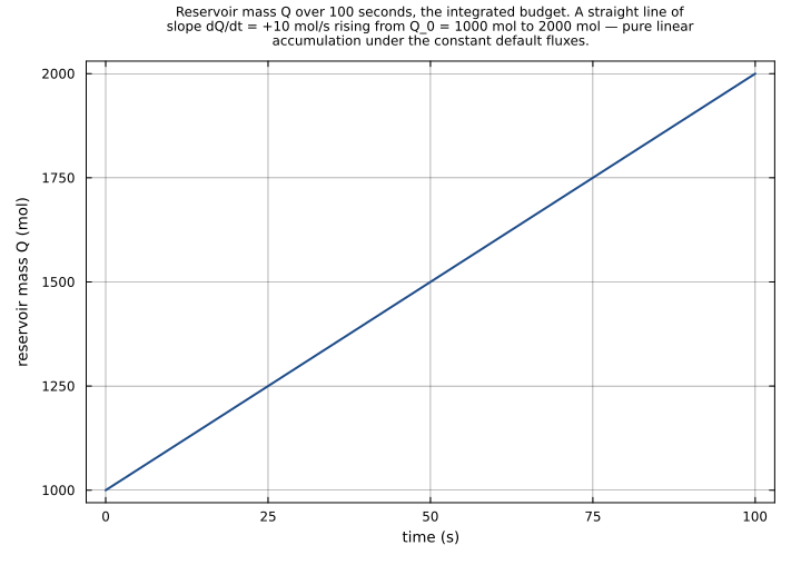
Observability classification: this component has exactly one differential state. Q carries the only D(·) operator; net_transport and net_chemistry are purely algebraic. Under constant flux inputs the budget equation D(Q) ~ (F_in - F_out) + (P - R_removal) has a constant right-hand side, so the analytic trajectory is the exact straight line Q(t) = Q_0 + [(F_in - F_out) + (P - R_removal)]·t, and net_transport, net_chemistry are constant in time. Test and example scenarios use time_span: [0.0, 100.0] so the linear accumulation/depletion/steady-state behaviour develops over a measurable range.
Numerical defaults: the upstream @variables carry no defaults — the .esm defaults are taken from the canonical upstream test scenario 2.1 Eq. 2.1: Mass Conservation (test/atmospheric_lifetime_test.jl:146-162): F_in = 100 mol/s, F_out = 80 mol/s, P = 50 mol/s, R_removal = 60 mol/s, at which dQ/dt = (100-80) + (50-60) = 10 mol/s, net_transport = 20 mol/s, net_chemistry = -10 mol/s. The reservoir initial mass Q_0 is not pinned by any AtmosphericBudget upstream test (its tests 2.1/2.2 are pure-arithmetic checks and 4.1 is a bare compilation check, none of which integrates a trajectory); the .esm adopts Q_0 = 1000 mol — a clean reference burden chosen so the default-scenario trajectory Q(t) = 1000 + 10·t doubles over the 100-second window, making the mass-conservation dynamics clearly measurable rather than lost beneath the reservoir magnitude.
Tolerance rationale (model-level rel=1.0e-10 / abs=1.0e-12): the budget equation is a non-stiff linear ODE with a constant right-hand side, and the two diagnostics are single-subtraction algebraic expressions. A constant-derivative ODE D(Q) = c is integrated exactly (up to floating-point round-off) by every consistent Runge-Kutta or Adams method — the analytic Q(t) = Q_0 + c·t is recovered to within a few ULP — and the inline-test gate’s numpy.interp sampling of a linear trajectory between solver output points is itself exact. The diagnostics F_in - F_out and P - R_removal are correctly-rounded single subtractions. rel=1.0e-10 therefore leaves several orders of magnitude of head-room above the realised round-off while still being a tight regression gate; the abs=1.0e-12 floor gates the exact-IEEE-754-zero diagnostic outputs that arise at the term-isolation boundaries (net_chemistry = 0 when P = R_removal = 0; net_transport = 0 when F_in = F_out = 0), catching the stuck-at-non-zero failure mode. This matches the observed-only sibling tolerance (ope.esm, co_oxidation.esm, oh_production.esm all rel=1e-10/abs=1e-12) and is far tighter than the stiff 18-state methane_ode.esm (rel=1e-6).
Upstream test reproduction (test/atmospheric_lifetime_test.jl):
1.1 AtmosphericBudget Structure(lines 19-40, asserts all 7 variable names present andlength(equations) == 3) — reproduced by the structural shape of the.esm: 7variablesentries (4 type:parameter + 3 type:state) and 3equationsentries; thedefaults_initial_state_and_diagnosticstest exercises all three state/diagnostic variables (Q, net_transport, net_chemistry) at t=0.2.1 Eq. 2.1: Mass Conservation(lines 146-162, the pure-arithmetic check F_in=100/F_out=80/P=50/R=60 ⇒ expected_dQdt = 10, net_transport = 20, net_chemistry = -10) — reproduced and tightened byupstream_mass_conservation_default_scenario, which runs the budget at exactly that scenario and pins net_transport = 20 and net_chemistry = -10 directly, and pins Q at t=0/10/50/100 so the slope Q(t) - Q(0) = 10·t reproduces the upstream dQ/dt = 10 as a structural fact of the integrated trajectory.2.2 Eq. 2.2: Steady State Condition(lines 165-178, the pure-arithmetic check that R_steady = F_in + P - F_out = 70 gives (F_in-F_out) + (P-R_steady) = 0) — reproduced byupstream_steady_state_zero_net_flux, which overrides R_removal to 70 and pins Q constant at 1000 over the whole window (dQ/dt = 0, the steady state) together with net_transport = 20 and net_chemistry = -20 (so net_transport + net_chemistry = 0, i.e. F_in + P = F_out + R_removal).4.1 AtmosphericBudget Compilation(lines 311-324,mtkcompile(budget; inputs = [F_in, F_out, P, R])succeeds) — reproduced structurally by encoding F_in, F_out, P, R_removal astype: parameter(the ESS analog of MTK inputs); every inline test below compiles and integrates the model through the canonical runner, which exercises the same compile path. The remaining tests extend coverage beyond the thin upstream suite: transport-only accumulation (P = R_removal = 0), chemistry-only decay (F_in = F_out = 0), production-dominated strong growth, removal-dominated decay from an elevated initial burden (exercising aninitial_conditionsoverride of Q_0), the fully-static null case (all four fluxes zero), and two diagnostic-isolation tests confirming net_transport responds only to F_in/F_out and net_chemistry only to P/R_removal.
Unit balance (verified): all three equations balance dimensionally.
D(Q) (F_in - F_out) + (P - R_removal): d/dt of mol is mol/s; each flux term is mol/s ✓
net_transport F_in - F_out: mol/s - mol/s = mol/s ✓
net_chemistry P - R_removal: mol/s - mol/s = mol/s ✓
Reservoir mass in mol, all fluxes and diagnostics in mol/s. SI throughout; no unit conversion at parse or runtime._
Variables
| Name | Units | Default | Description |
|---|---|---|---|
Q | mol | 1000.0 | Total mass (amount of substance) of the species held in the reservoir [mol] (S&P Ch. 2 Eq. 2.1). The single differential (integrated) state of the component: its governing equation is the budget ODE D(Q) ~ (F_in - F_out) + (P - R_removal). The default 1000 mol is the t=0 initial condition Q_0; it is not pinned by any upstream AtmosphericBudget test (the upstream 2.1/2.2 tests are pure arithmetic and 4.1 is a bare compilation check), and is chosen as a clean reference burden so the default-scenario trajectory Q(t) = 1000 + 10·t doubles over the 100 s window. Under constant flux inputs Q evolves linearly; it rises when the net flux (F_in - F_out) + (P - R_removal) is positive (accumulation), holds steady when it is zero (S&P Eq. 2.2 steady state), and falls when it is negative (depletion). Overridable per scenario via initial_conditions. |
Parameters
| Name | Units | Default | Description |
|---|---|---|---|
F_in | mol/s | 100.0 | Rate of mass inflow into the reservoir from outside [mol/s] (S&P Ch. 2 Eq. 2.1, externally-supplied transport input). The default 100 mol/s is the value used in the canonical upstream test scenario 2.1 Eq. 2.1: Mass Conservation (test/atmospheric_lifetime_test.jl:148). F_in raises the reservoir mass and is one of the two terms of the net transport diagnostic net_transport = F_in - F_out. Encoded as type: parameter (not type: state) because AtmosphericBudget has no governing equation for F_in — it is purely an input, supplied via parameter_overrides in tests and parameter_sweep in examples; the upstream model treats it as an mtkcompile input. |
F_out | mol/s | 80.0 | Rate of mass outflow from the reservoir [mol/s] (S&P Ch. 2 Eq. 2.1, externally-supplied transport input). The default 80 mol/s is the value used in the canonical upstream test scenario 2.1 Eq. 2.1: Mass Conservation (test/atmospheric_lifetime_test.jl:149). F_out lowers the reservoir mass and is the subtracted term of the net transport diagnostic net_transport = F_in - F_out. Encoded as type: parameter (externally-supplied input with no governing equation in this component). |
P | mol/s | 50.0 | Rate of chemical production within the reservoir [mol/s] (S&P Ch. 2 Eq. 2.1, externally-supplied chemistry input). The default 50 mol/s is the value used in the canonical upstream test scenario 2.1 Eq. 2.1: Mass Conservation (test/atmospheric_lifetime_test.jl:150). P raises the reservoir mass and is the first term of the net chemistry diagnostic net_chemistry = P - R_removal. Kept as the bare upstream name P (unlike the removal rate, P is not a reserved physical-constant name in the ESS schema). Encoded as type: parameter (externally-supplied input with no governing equation in this component). |
R_removal | mol/s | 60.0 | Rate of chemical removal within the reservoir [mol/s] (S&P Ch. 2 Eq. 2.1, externally-supplied chemistry input; the upstream @variable R, renamed here — see model reference notes — because the ESS schema reserves R for the ideal gas constant). The default 60 mol/s is the value used in the canonical upstream test scenario 2.1 Eq. 2.1: Mass Conservation (test/atmospheric_lifetime_test.jl:151). R_removal lowers the reservoir mass and is the subtracted term of the net chemistry diagnostic net_chemistry = P - R_removal. The steady-state condition (S&P Eq. 2.2) dQ/dt = 0 is reached at R_removal = F_in + P - F_out = 70 mol/s for the default fluxes. Encoded as type: parameter (externally-supplied input with no governing equation in this component). |
Observed
| Name | Units | Default | Description |
|---|---|---|---|
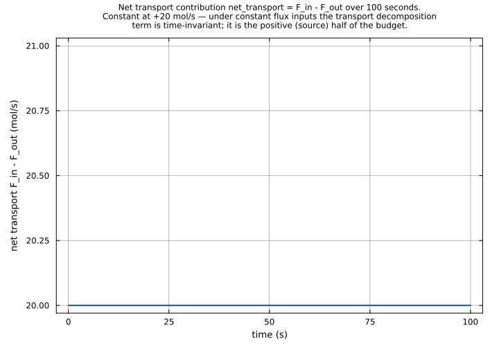
net_transport | mol/s | Net transport contribution to the reservoir budget [mol/s] (S&P Ch. 2, diagnostic on Eq. 2.1): net_transport = F_in - F_out, the inflow minus the outflow. An observed (algebraic) state — the LHS of one purely-algebraic equation, with no time derivative and hence no initial condition. At the default scenario net_transport = 100 - 80 = 20 mol/s. Together with net_chemistry it decomposes the budget: D(Q) = net_transport + net_chemistry. Depends only on the transport inputs F_in and F_out, never on the chemistry inputs P, R_removal. | |
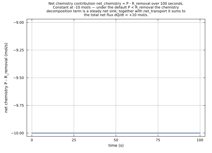
net_chemistry | mol/s | Net chemistry contribution to the reservoir budget [mol/s] (S&P Ch. 2, diagnostic on Eq. 2.1): net_chemistry = P - R_removal, the chemical production minus the chemical removal. An observed (algebraic) state — the LHS of one purely-algebraic equation, with no time derivative and hence no initial condition. At the default scenario net_chemistry = 50 - 60 = -10 mol/s (a net chemical sink). Together with net_transport it decomposes the budget: D(Q) = net_transport + net_chemistry; the steady-state condition (S&P Eq. 2.2) is net_chemistry = -net_transport. Depends only on the chemistry inputs P and R_removal, never on the transport inputs F_in, F_out. |
Observed expressions
$$ net_{transport} = F_{in} + \left(-1.0\right) \cdot F_{out} $$Net transport contribution to the reservoir budget [mol/s] (S&P Ch. 2, diagnostic on Eq. 2.1): net_transport = F_in - F_out, the inflow minus the outflow. An observed (algebraic) state — the LHS of one purely-algebraic equation, with no time derivative and hence no initial condition. At the default scenario net_transport = 100 - 80 = 20 mol/s. Together with net_chemistry it decomposes the budget: D(Q) = net_transport + net_chemistry. Depends only on the transport inputs F_in and F_out, never on the chemistry inputs P, R_removal.
$$ net_{chemistry} = P + \left(-1.0\right) \cdot R_{removal} $$Net chemistry contribution to the reservoir budget [mol/s] (S&P Ch. 2, diagnostic on Eq. 2.1): net_chemistry = P - R_removal, the chemical production minus the chemical removal. An observed (algebraic) state — the LHS of one purely-algebraic equation, with no time derivative and hence no initial condition. At the default scenario net_chemistry = 50 - 60 = -10 mol/s (a net chemical sink). Together with net_transport it decomposes the budget: D(Q) = net_transport + net_chemistry; the steady-state condition (S&P Eq. 2.2) is net_chemistry = -net_transport. Depends only on the chemistry inputs P and R_removal, never on the transport inputs F_in, F_out.
Equations
$$ \mathrm{D}\left(Q\right) = F_{in} + \left(-1.0\right) \cdot F_{out} + P + \left(-1.0\right) \cdot R_{removal} $$Analyses
default_mass_budget_run
Headline 100-second integration of the reservoir budget under the canonical default scenario (Q_0 = 1000 mol, F_in = 100, F_out = 80, P = 50, R_removal = 60 mol/s — the upstream 2.1 Eq. 2.1: Mass Conservation fluxes). The net transport (+20 mol/s) outweighs the net chemistry (-10 mol/s), giving a total net flux of +10 mol/s, so the reservoir mass accumulates linearly, doubling from 1000 to 2000 mol over the window. Plots the integrated reservoir mass Q(t) and the two time-invariant diagnostic decomposition terms net_transport(t) and net_chemistry(t), the visual statement of S&P Eq. 2.1 dQ/dt = (F_in - F_out) + (P - R_removal).
Time span: 0.0 → 100.0
removal_rate_regime_sweep
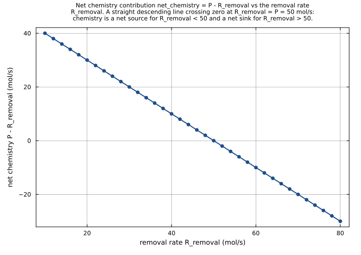
Removal-rate regime sweep: the chemical removal R_removal is swept linearly over [10, 80] mol/s with the other fluxes at their defaults (F_in=100, F_out=80, P=50) and Q_0 = 1000 mol, integrating the budget over 100 s at each grid point. The net flux is (F_in-F_out) + (P-R_removal) = 70 - R_removal, so the final reservoir mass is Q(100) = 1000 + 100·(70-R_removal): the reservoir accumulates for R_removal < 70, holds at its initial 1000 mol at exactly R_removal = 70 (the S&P Eq. 2.2 steady state), and begins to deplete for R_removal > 70. Surfaces how the chemical sink controls the budget — the removal-side analog of the production sweep.
Time span: 0.0 → 100.0
Swept over: R_removal

production_rate_regime_sweep
Production-rate regime sweep: the chemical production P is swept linearly over [30, 130] mol/s with the other fluxes at their defaults (F_in=100, F_out=80, R_removal=60) and Q_0 = 1000 mol, integrating the budget over 100 s at each grid point. The net flux is (F_in-F_out) + (P-R_removal) = P - 40, so the final reservoir mass is Q(100) = 1000 + 100·(P-40): the reservoir holds at its initial 1000 mol at exactly P = 40 (the S&P Eq. 2.2 steady state) and accumulates ever more steeply as P rises. Surfaces how the chemical source controls the budget — the production-side analog of the removal sweep.
Time span: 0.0 → 100.0
Swept over: P


Raw .esm
Raw .esm JSON (this component)
{
"reference": {
"notes": "source_ref: GasChem.jl@8c12c048482b515fb8eb2110bf8ab4b4f4e71309:src/AtmosphericLifetime.jl:64\n\nUpstream `AtmosphericBudget` is an MTK `@component` with 7 `@variables` (Q, F_in, F_out, P, R, net_transport, net_chemistry), 0 `@parameters`, 0 `@constants`, and 3 equations from S&P Ch. 2 Eqs. 2.1-2.2. It is the simplest component of the AtmosphericLifetime module — the bare reservoir mass-balance on which SpeciesLifetime, MultipleRemovalLifetime, OHReactionLifetime and TroposphericBudget (the other four components of the same source file) elaborate. The upstream test compiles the system with `mtkcompile(budget; inputs = [F_in, F_out, P, R])` (test/atmospheric_lifetime_test.jl `4.1 AtmosphericBudget Compilation`, lines 311-324), pinning the four flux terms as externally-supplied inputs and integrating the single differential state Q.\n\nVariable rename — `R` → `R_removal`: the upstream removal-rate @variable is named `R`. The ESS schema validator reserves the bare name `R` for the ideal gas constant (`earthsci_ast.parse._KNOWN_PHYSICAL_CONSTANTS = {R, k_B, N_A}`) and rejects any `type: parameter` named `R` whose units are not dimensionally compatible with J/(mol*K). The removal rate is mol/s, so the migration renames it `R_removal` (a name that records its physical role — chemical removal rate — and cannot collide with the reserved set). This is the only variable renamed; Q, F_in, F_out, P, net_transport and net_chemistry are preserved verbatim from the upstream `@variables`. `P` (chemical production rate) is NOT reserved and is kept as-is.\n\nVariable-classification convention: the four flux @variables F_in, F_out, P, R_removal are encoded here as `type: parameter` because they have no defining equation within the AtmosphericBudget component itself — they are externally-supplied inputs that the upstream compile treats via `mtkcompile(...; inputs = [...])`. This mirrors the rig-wide convention applied by sibling co_oxidation.esm (its six input @variables CO/OH/HO2/NO/NO2/O3 are encoded as `type: parameter`), ope.esm and oh_production.esm. Of the remaining three @variables, Q is encoded as `type: state` with a `default` because it is a genuine differential (integrated) state — its defining equation is the ODE `D(Q) ~ ...` and the `default` supplies the t=0 initial condition (the same convention as every species in sibling methane_ode.esm). net_transport and net_chemistry are encoded as `type: state` without a `default` because each is the LHS of exactly one purely-algebraic equation — they are observed (diagnostic) variables fully determined at every instant by the inputs, with no integration and hence no initial condition (the same convention as the observed outputs P_O3/L_NOx/OPE of sibling ope.esm). The upstream structural test `1.1 AtmosphericBudget Structure` (test/atmospheric_lifetime_test.jl:19-40) asserts that all 7 variable names appear in `unknowns(budget)` (pre-`mtkcompile`, when inputs are still unknowns) and `length(equations(budget)) == 3` — the .esm preserves this with 7 declared `variables` entries (4 parameter + 3 state) and 3 entries in `equations`.\n\nUnits: the upstream Julia declares Q in `u\"mol\"` and F_in/F_out/P/R/net_transport/net_chemistry in `u\"mol/s\"`. These are already SI-coherent (the mole is the SI base unit of amount of substance, the second the SI base unit of time) — unlike the CGS rate constants of the chemistry-mechanism siblings, no unit conversion is applied at migration time. The `.esm` carries `mol` and `mol/s` verbatim. AtmosphericBudget is a generic single-reservoir budget; Q, the four fluxes and the two diagnostics share the textbook's mole/mole-per-second units and carry no species-specific normalization.\n\nEquation faithfulness: the upstream `eqs` array (src/AtmosphericLifetime.jl:78-85) is `[D(Q) ~ (F_in - F_out) + (P - R), net_transport ~ F_in - F_out, net_chemistry ~ P - R]`. The `.esm` `equations` array preserves this order verbatim (with `R` → `R_removal`). The D(Q) right-hand side is written in terms of the raw flux inputs F_in, F_out, P, R_removal — NOT in terms of the diagnostic variables net_transport and net_chemistry — exactly as the upstream writes it; although `D(Q)` numerically equals `net_transport + net_chemistry`, the upstream keeps the budget equation independent of the two diagnostic variables, and the migration is faithful to that. Subtraction is encoded in the rig-wide additive-with-negated-product idiom (a `-1.0` literal multiplier inside a `*` node, summed by a `+` node) used by sibling methane_ode.esm; `(F_in - F_out) + (P - R_removal)` flattens by associativity of `+` to the single 4-term sum `F_in + (-1·F_out) + P + (-1·R_removal)`, which the ESS canonicalizer treats identically to any parenthesized grouping. No equation references another equation's LHS, so the verbatim upstream order (D(Q), net_transport, net_chemistry) is already a valid evaluation order.\n\nObservability classification: this component has exactly one differential state. Q carries the only `D(·)` operator; net_transport and net_chemistry are purely algebraic. Under constant flux inputs the budget equation `D(Q) ~ (F_in - F_out) + (P - R_removal)` has a constant right-hand side, so the analytic trajectory is the exact straight line Q(t) = Q_0 + [(F_in - F_out) + (P - R_removal)]·t, and net_transport, net_chemistry are constant in time. Test and example scenarios use `time_span: [0.0, 100.0]` so the linear accumulation/depletion/steady-state behaviour develops over a measurable range.\n\nNumerical defaults: the upstream @variables carry no defaults — the `.esm` defaults are taken from the canonical upstream test scenario `2.1 Eq. 2.1: Mass Conservation` (test/atmospheric_lifetime_test.jl:146-162): F_in = 100 mol/s, F_out = 80 mol/s, P = 50 mol/s, R_removal = 60 mol/s, at which dQ/dt = (100-80) + (50-60) = 10 mol/s, net_transport = 20 mol/s, net_chemistry = -10 mol/s. The reservoir initial mass Q_0 is not pinned by any AtmosphericBudget upstream test (its tests `2.1`/`2.2` are pure-arithmetic checks and `4.1` is a bare compilation check, none of which integrates a trajectory); the `.esm` adopts Q_0 = 1000 mol — a clean reference burden chosen so the default-scenario trajectory Q(t) = 1000 + 10·t doubles over the 100-second window, making the mass-conservation dynamics clearly measurable rather than lost beneath the reservoir magnitude.\n\nTolerance rationale (model-level rel=1.0e-10 / abs=1.0e-12): the budget equation is a non-stiff linear ODE with a constant right-hand side, and the two diagnostics are single-subtraction algebraic expressions. A constant-derivative ODE `D(Q) = c` is integrated exactly (up to floating-point round-off) by every consistent Runge-Kutta or Adams method — the analytic Q(t) = Q_0 + c·t is recovered to within a few ULP — and the inline-test gate's `numpy.interp` sampling of a linear trajectory between solver output points is itself exact. The diagnostics F_in - F_out and P - R_removal are correctly-rounded single subtractions. rel=1.0e-10 therefore leaves several orders of magnitude of head-room above the realised round-off while still being a tight regression gate; the abs=1.0e-12 floor gates the exact-IEEE-754-zero diagnostic outputs that arise at the term-isolation boundaries (net_chemistry = 0 when P = R_removal = 0; net_transport = 0 when F_in = F_out = 0), catching the stuck-at-non-zero failure mode. This matches the observed-only sibling tolerance (ope.esm, co_oxidation.esm, oh_production.esm all rel=1e-10/abs=1e-12) and is far tighter than the stiff 18-state methane_ode.esm (rel=1e-6).\n\nUpstream test reproduction (test/atmospheric_lifetime_test.jl):\n- `1.1 AtmosphericBudget Structure` (lines 19-40, asserts all 7 variable names present and `length(equations) == 3`) — reproduced by the structural shape of the `.esm`: 7 `variables` entries (4 type:parameter + 3 type:state) and 3 `equations` entries; the `defaults_initial_state_and_diagnostics` test exercises all three state/diagnostic variables (Q, net_transport, net_chemistry) at t=0.\n- `2.1 Eq. 2.1: Mass Conservation` (lines 146-162, the pure-arithmetic check F_in=100/F_out=80/P=50/R=60 ⇒ expected_dQdt = 10, net_transport = 20, net_chemistry = -10) — reproduced and tightened by `upstream_mass_conservation_default_scenario`, which runs the budget at exactly that scenario and pins net_transport = 20 and net_chemistry = -10 directly, and pins Q at t=0/10/50/100 so the slope Q(t) - Q(0) = 10·t reproduces the upstream dQ/dt = 10 as a structural fact of the integrated trajectory.\n- `2.2 Eq. 2.2: Steady State Condition` (lines 165-178, the pure-arithmetic check that R_steady = F_in + P - F_out = 70 gives (F_in-F_out) + (P-R_steady) = 0) — reproduced by `upstream_steady_state_zero_net_flux`, which overrides R_removal to 70 and pins Q constant at 1000 over the whole window (dQ/dt = 0, the steady state) together with net_transport = 20 and net_chemistry = -20 (so net_transport + net_chemistry = 0, i.e. F_in + P = F_out + R_removal).\n- `4.1 AtmosphericBudget Compilation` (lines 311-324, `mtkcompile(budget; inputs = [F_in, F_out, P, R])` succeeds) — reproduced structurally by encoding F_in, F_out, P, R_removal as `type: parameter` (the ESS analog of MTK inputs); every inline test below compiles and integrates the model through the canonical runner, which exercises the same compile path.\nThe remaining tests extend coverage beyond the thin upstream suite: transport-only accumulation (P = R_removal = 0), chemistry-only decay (F_in = F_out = 0), production-dominated strong growth, removal-dominated decay from an elevated initial burden (exercising an `initial_conditions` override of Q_0), the fully-static null case (all four fluxes zero), and two diagnostic-isolation tests confirming net_transport responds only to F_in/F_out and net_chemistry only to P/R_removal.\n\nUnit balance (verified): all three equations balance dimensionally.\n D(Q) `(F_in - F_out) + (P - R_removal)`: d/dt of mol is mol/s; each flux term is mol/s ✓\n net_transport `F_in - F_out`: mol/s - mol/s = mol/s ✓\n net_chemistry `P - R_removal`: mol/s - mol/s = mol/s ✓\nReservoir mass in mol, all fluxes and diagnostics in mol/s. SI throughout; no unit conversion at parse or runtime."
},
"tolerance": {
"rel": 1e-10,
"abs": 1e-12
},
"variables": {
"F_in": {
"type": "parameter",
"units": "mol/s",
"default": 100.0,
"description": "Rate of mass inflow into the reservoir from outside [mol/s] (S&P Ch. 2 Eq. 2.1, externally-supplied transport input). The default 100 mol/s is the value used in the canonical upstream test scenario `2.1 Eq. 2.1: Mass Conservation` (test/atmospheric_lifetime_test.jl:148). F_in raises the reservoir mass and is one of the two terms of the net transport diagnostic net_transport = F_in - F_out. Encoded as `type: parameter` (not `type: state`) because AtmosphericBudget has no governing equation for F_in — it is purely an input, supplied via `parameter_overrides` in tests and `parameter_sweep` in examples; the upstream model treats it as an `mtkcompile` input."
},
"F_out": {
"type": "parameter",
"units": "mol/s",
"default": 80.0,
"description": "Rate of mass outflow from the reservoir [mol/s] (S&P Ch. 2 Eq. 2.1, externally-supplied transport input). The default 80 mol/s is the value used in the canonical upstream test scenario `2.1 Eq. 2.1: Mass Conservation` (test/atmospheric_lifetime_test.jl:149). F_out lowers the reservoir mass and is the subtracted term of the net transport diagnostic net_transport = F_in - F_out. Encoded as `type: parameter` (externally-supplied input with no governing equation in this component)."
},
"P": {
"type": "parameter",
"units": "mol/s",
"default": 50.0,
"description": "Rate of chemical production within the reservoir [mol/s] (S&P Ch. 2 Eq. 2.1, externally-supplied chemistry input). The default 50 mol/s is the value used in the canonical upstream test scenario `2.1 Eq. 2.1: Mass Conservation` (test/atmospheric_lifetime_test.jl:150). P raises the reservoir mass and is the first term of the net chemistry diagnostic net_chemistry = P - R_removal. Kept as the bare upstream name `P` (unlike the removal rate, `P` is not a reserved physical-constant name in the ESS schema). Encoded as `type: parameter` (externally-supplied input with no governing equation in this component)."
},
"R_removal": {
"type": "parameter",
"units": "mol/s",
"default": 60.0,
"description": "Rate of chemical removal within the reservoir [mol/s] (S&P Ch. 2 Eq. 2.1, externally-supplied chemistry input; the upstream @variable `R`, renamed here — see model reference notes — because the ESS schema reserves `R` for the ideal gas constant). The default 60 mol/s is the value used in the canonical upstream test scenario `2.1 Eq. 2.1: Mass Conservation` (test/atmospheric_lifetime_test.jl:151). R_removal lowers the reservoir mass and is the subtracted term of the net chemistry diagnostic net_chemistry = P - R_removal. The steady-state condition (S&P Eq. 2.2) dQ/dt = 0 is reached at R_removal = F_in + P - F_out = 70 mol/s for the default fluxes. Encoded as `type: parameter` (externally-supplied input with no governing equation in this component)."
},
"Q": {
"type": "unknown",
"units": "mol",
"default": 1000.0,
"description": "Total mass (amount of substance) of the species held in the reservoir [mol] (S&P Ch. 2 Eq. 2.1). The single differential (integrated) state of the component: its governing equation is the budget ODE D(Q) ~ (F_in - F_out) + (P - R_removal). The `default` 1000 mol is the t=0 initial condition Q_0; it is not pinned by any upstream AtmosphericBudget test (the upstream `2.1`/`2.2` tests are pure arithmetic and `4.1` is a bare compilation check), and is chosen as a clean reference burden so the default-scenario trajectory Q(t) = 1000 + 10·t doubles over the 100 s window. Under constant flux inputs Q evolves linearly; it rises when the net flux (F_in - F_out) + (P - R_removal) is positive (accumulation), holds steady when it is zero (S&P Eq. 2.2 steady state), and falls when it is negative (depletion). Overridable per scenario via `initial_conditions`."
},
"net_transport": {
"type": "unknown",
"units": "mol/s",
"description": "Net transport contribution to the reservoir budget [mol/s] (S&P Ch. 2, diagnostic on Eq. 2.1): net_transport = F_in - F_out, the inflow minus the outflow. An observed (algebraic) state — the LHS of one purely-algebraic equation, with no time derivative and hence no initial condition. At the default scenario net_transport = 100 - 80 = 20 mol/s. Together with net_chemistry it decomposes the budget: D(Q) = net_transport + net_chemistry. Depends only on the transport inputs F_in and F_out, never on the chemistry inputs P, R_removal."
},
"net_chemistry": {
"type": "unknown",
"units": "mol/s",
"description": "Net chemistry contribution to the reservoir budget [mol/s] (S&P Ch. 2, diagnostic on Eq. 2.1): net_chemistry = P - R_removal, the chemical production minus the chemical removal. An observed (algebraic) state — the LHS of one purely-algebraic equation, with no time derivative and hence no initial condition. At the default scenario net_chemistry = 50 - 60 = -10 mol/s (a net chemical sink). Together with net_transport it decomposes the budget: D(Q) = net_transport + net_chemistry; the steady-state condition (S&P Eq. 2.2) is net_chemistry = -net_transport. Depends only on the chemistry inputs P and R_removal, never on the transport inputs F_in, F_out."
}
},
"equations": [
{
"lhs": {
"op": "D",
"wrt": "t",
"args": [
"Q"
]
},
"rhs": {
"op": "+",
"args": [
"F_in",
{
"op": "*",
"args": [
-1.0,
"F_out"
]
},
"P",
{
"op": "*",
"args": [
-1.0,
"R_removal"
]
}
]
}
},
{
"lhs": "net_transport",
"rhs": {
"op": "+",
"args": [
"F_in",
{
"op": "*",
"args": [
-1.0,
"F_out"
]
}
]
}
},
{
"lhs": "net_chemistry",
"rhs": {
"op": "+",
"args": [
"P",
{
"op": "*",
"args": [
-1.0,
"R_removal"
]
}
]
}
}
],
"tests": [
{
"id": "defaults_initial_state_and_diagnostics",
"description": "Initial state and diagnostic decomposition at t=0 under the declared defaults (F_in=100, F_out=80, P=50, R_removal=60, Q_0=1000). Reproduces the upstream structural test `1.1 AtmosphericBudget Structure` (test/atmospheric_lifetime_test.jl:19-40) by exercising all three state/diagnostic variables — the integrated reservoir mass Q at its initial condition (1000 mol) and the two observed diagnostics net_transport = F_in - F_out = 20 and net_chemistry = P - R_removal = -10. At t=0 there is no integration drift, so this pins the parser-to-Float64 conversion of the declared defaults and the first-instant evaluation of the two algebraic equations.",
"parameter_overrides": {},
"time_span": {
"start": 0.0,
"end": 100.0
},
"assertions": [
{
"variable": "Q",
"time": 0.0,
"expected": 1000.0
},
{
"variable": "net_transport",
"time": 0.0,
"expected": 20.0
},
{
"variable": "net_chemistry",
"time": 0.0,
"expected": -10.0
}
]
},
{
"id": "upstream_mass_conservation_default_scenario",
"description": "Reproduces and tightens the upstream `2.1 Eq. 2.1: Mass Conservation` test (test/atmospheric_lifetime_test.jl:146-162). At the canonical scenario F_in=100, F_out=80, P=50, R_removal=60 — every flux at its declared default — the upstream asserts dQ/dt = (F_in-F_out) + (P-R) = 10, net_transport = 20, net_chemistry = -10. This test pins net_transport = 20 and net_chemistry = -10 directly (constant in time, sampled at both ends of the window), and pins the integrated reservoir mass Q at t=0/10/50/100: the linear trajectory Q(t) = 1000 + 10·t passes through 1000, 1100, 1500, 2000, so the realised slope reproduces the upstream dQ/dt = 10 mol/s as a structural fact of the integrated solution rather than a hand-arithmetic check.",
"parameter_overrides": {},
"time_span": {
"start": 0.0,
"end": 100.0
},
"assertions": [
{
"variable": "Q",
"time": 0.0,
"expected": 1000.0
},
{
"variable": "Q",
"time": 10.0,
"expected": 1100.0
},
{
"variable": "Q",
"time": 50.0,
"expected": 1500.0
},
{
"variable": "Q",
"time": 100.0,
"expected": 2000.0
},
{
"variable": "net_transport",
"time": 0.0,
"expected": 20.0
},
{
"variable": "net_transport",
"time": 100.0,
"expected": 20.0
},
{
"variable": "net_chemistry",
"time": 0.0,
"expected": -10.0
},
{
"variable": "net_chemistry",
"time": 100.0,
"expected": -10.0
}
]
},
{
"id": "upstream_steady_state_zero_net_flux",
"description": "Reproduces the upstream `2.2 Eq. 2.2: Steady State Condition` test (test/atmospheric_lifetime_test.jl:165-178). The upstream computes the removal rate R_steady = F_in + P - F_out = 100 + 50 - 80 = 70 mol/s at which dQ/dt vanishes. This test overrides R_removal to 70 (F_in/F_out/P at defaults) so the net flux (F_in-F_out) + (P-R_removal) = 20 + (50-70) = 0: the reservoir mass Q holds exactly constant at its initial 1000 mol over the whole window, the textbook steady state. net_transport = 20 and net_chemistry = P - R_removal = -20 are equal and opposite (net_transport + net_chemistry = 0), the diagnostic form of the steady-state identity F_in + P = F_out + R_removal.",
"parameter_overrides": {
"R_removal": 70.0
},
"time_span": {
"start": 0.0,
"end": 100.0
},
"assertions": [
{
"variable": "Q",
"time": 0.0,
"expected": 1000.0
},
{
"variable": "Q",
"time": 50.0,
"expected": 1000.0
},
{
"variable": "Q",
"time": 100.0,
"expected": 1000.0
},
{
"variable": "net_transport",
"time": 50.0,
"expected": 20.0
},
{
"variable": "net_chemistry",
"time": 50.0,
"expected": -20.0
}
]
},
{
"id": "transport_only_pure_accumulation",
"description": "Transport-only regime: the chemistry inputs are zeroed (P = R_removal = 0) so net_chemistry = 0 and the budget is driven entirely by transport. dQ/dt = net_transport = F_in - F_out = 20 mol/s, a pure linear accumulation: Q(t) = 1000 + 20·t passes through 1000, 2000, 3000 at t=0/50/100. Isolates the transport term of Eq. 2.1 and confirms that with no chemistry the reservoir grows at exactly the net transport rate. The net_chemistry = 0 assertion uses a pure absolute tolerance to gate the exact-IEEE-754-zero output against a stuck-at-non-zero regression.",
"parameter_overrides": {
"P": 0.0,
"R_removal": 0.0
},
"time_span": {
"start": 0.0,
"end": 100.0
},
"assertions": [
{
"variable": "Q",
"time": 0.0,
"expected": 1000.0
},
{
"variable": "Q",
"time": 50.0,
"expected": 2000.0
},
{
"variable": "Q",
"time": 100.0,
"expected": 3000.0
},
{
"variable": "net_transport",
"time": 50.0,
"expected": 20.0
},
{
"variable": "net_chemistry",
"time": 50.0,
"expected": 0.0,
"tolerance": {
"abs": 1e-12
}
}
]
},
{
"id": "chemistry_only_pure_decay",
"description": "Chemistry-only regime: the transport inputs are zeroed (F_in = F_out = 0) so net_transport = 0 and the budget is driven entirely by chemistry. With the default P=50 < R_removal=60 the net chemistry is a sink, dQ/dt = net_chemistry = P - R_removal = -10 mol/s, a pure linear decay: Q(t) = 1000 - 10·t passes through 1000, 500, 100 at t=0/50/90 (sampled short of the t=100 reservoir-exhaustion point). Isolates the chemistry term of Eq. 2.1 and confirms that with no transport the reservoir drains at exactly the net chemical loss rate. The net_transport = 0 assertion uses a pure absolute tolerance to gate the exact-IEEE-754-zero output.",
"parameter_overrides": {
"F_in": 0.0,
"F_out": 0.0
},
"time_span": {
"start": 0.0,
"end": 100.0
},
"assertions": [
{
"variable": "Q",
"time": 0.0,
"expected": 1000.0
},
{
"variable": "Q",
"time": 50.0,
"expected": 500.0
},
{
"variable": "Q",
"time": 90.0,
"expected": 100.0
},
{
"variable": "net_transport",
"time": 50.0,
"expected": 0.0,
"tolerance": {
"abs": 1e-12
}
},
{
"variable": "net_chemistry",
"time": 50.0,
"expected": -10.0
}
]
},
{
"id": "production_dominated_strong_growth",
"description": "Production-dominated regime: the chemical production P is raised to 200 mol/s (F_in/F_out/R_removal at defaults), making net_chemistry = P - R_removal = 140 mol/s a strong net source. The total net flux is (F_in-F_out) + (P-R_removal) = 20 + 140 = 160 mol/s, so the reservoir grows steeply: Q(t) = 1000 + 160·t passes through 1000, 5000, 17000 at t=0/25/100. Exercises the strong-source limb of the budget where chemical production dominates over both removal and net transport.",
"parameter_overrides": {
"P": 200.0
},
"time_span": {
"start": 0.0,
"end": 100.0
},
"assertions": [
{
"variable": "Q",
"time": 0.0,
"expected": 1000.0
},
{
"variable": "Q",
"time": 25.0,
"expected": 5000.0
},
{
"variable": "Q",
"time": 100.0,
"expected": 17000.0
},
{
"variable": "net_transport",
"time": 50.0,
"expected": 20.0
},
{
"variable": "net_chemistry",
"time": 50.0,
"expected": 140.0
}
]
},
{
"id": "removal_dominated_decay_high_burden",
"description": "Removal-dominated regime from an elevated initial burden: the chemical removal R_removal is raised to 200 mol/s (F_in/F_out/P at defaults) and the initial reservoir mass Q_0 is overridden to 20000 mol via `initial_conditions`. net_chemistry = P - R_removal = -150 mol/s is a strong sink; the total net flux is 20 + (50-200) = -130 mol/s, so the reservoir drains linearly: Q(t) = 20000 - 130·t passes through 20000, 13500, 7000 at t=0/50/100 (the elevated Q_0 keeps the trajectory positive over the whole window). Exercises the strong-sink limb of the budget and, via the Q_0 override, the `initial_conditions` pathway.",
"parameter_overrides": {
"R_removal": 200.0
},
"initial_conditions": {
"Q": 20000.0
},
"time_span": {
"start": 0.0,
"end": 100.0
},
"assertions": [
{
"variable": "Q",
"time": 0.0,
"expected": 20000.0
},
{
"variable": "Q",
"time": 50.0,
"expected": 13500.0
},
{
"variable": "Q",
"time": 100.0,
"expected": 7000.0
},
{
"variable": "net_transport",
"time": 50.0,
"expected": 20.0
},
{
"variable": "net_chemistry",
"time": 50.0,
"expected": -150.0
}
]
},
{
"id": "all_fluxes_zero_static_reservoir",
"description": "Fully-static null case: all four flux inputs are zeroed (F_in = F_out = P = R_removal = 0). The net transport, net chemistry and total net flux all vanish, so the reservoir mass Q holds exactly constant at its initial 1000 mol for all time — a closed reservoir with neither transport nor chemistry. Sentinel test confirming that the budget ODE has no spurious source or sink term: any constant added to the D(Q) right-hand side would drift Q off 1000. The net_transport = 0 and net_chemistry = 0 assertions use pure absolute tolerances to gate the exact-IEEE-754-zero outputs.",
"parameter_overrides": {
"F_in": 0.0,
"F_out": 0.0,
"P": 0.0,
"R_removal": 0.0
},
"time_span": {
"start": 0.0,
"end": 100.0
},
"assertions": [
{
"variable": "Q",
"time": 0.0,
"expected": 1000.0
},
{
"variable": "Q",
"time": 100.0,
"expected": 1000.0
},
{
"variable": "net_transport",
"time": 50.0,
"expected": 0.0,
"tolerance": {
"abs": 1e-12
}
},
{
"variable": "net_chemistry",
"time": 50.0,
"expected": 0.0,
"tolerance": {
"abs": 1e-12
}
}
]
},
{
"id": "transport_diagnostic_isolation",
"description": "Diagnostic-isolation test for the transport term: only the inflow F_in is perturbed (raised to 130 mol/s; F_out/P/R_removal at defaults). net_transport = F_in - F_out responds, rising to 130 - 80 = 50 mol/s, while net_chemistry = P - R_removal is unchanged at 50 - 60 = -10 mol/s — confirming the net chemistry diagnostic is wired only to the chemistry inputs and does not leak the transport perturbation. The total net flux is 50 + (-10) = 40 mol/s, so Q(t) = 1000 + 40·t reaches 5000 at t=100. Paired with `chemistry_diagnostic_isolation` to catch any cross-wiring between the two diagnostic equations.",
"parameter_overrides": {
"F_in": 130.0
},
"time_span": {
"start": 0.0,
"end": 100.0
},
"assertions": [
{
"variable": "Q",
"time": 0.0,
"expected": 1000.0
},
{
"variable": "Q",
"time": 100.0,
"expected": 5000.0
},
{
"variable": "net_transport",
"time": 50.0,
"expected": 50.0
},
{
"variable": "net_chemistry",
"time": 50.0,
"expected": -10.0
}
]
},
{
"id": "chemistry_diagnostic_isolation",
"description": "Diagnostic-isolation test for the chemistry term: only the removal R_removal is perturbed (lowered to 20 mol/s; F_in/F_out/P at defaults). net_chemistry = P - R_removal responds, rising to 50 - 20 = 30 mol/s, while net_transport = F_in - F_out is unchanged at 100 - 80 = 20 mol/s — confirming the net transport diagnostic is wired only to the transport inputs and does not leak the chemistry perturbation. The total net flux is 20 + 30 = 50 mol/s, so Q(t) = 1000 + 50·t reaches 6000 at t=100. Paired with `transport_diagnostic_isolation` to catch any cross-wiring between the two diagnostic equations.",
"parameter_overrides": {
"R_removal": 20.0
},
"time_span": {
"start": 0.0,
"end": 100.0
},
"assertions": [
{
"variable": "Q",
"time": 0.0,
"expected": 1000.0
},
{
"variable": "Q",
"time": 100.0,
"expected": 6000.0
},
{
"variable": "net_transport",
"time": 50.0,
"expected": 20.0
},
{
"variable": "net_chemistry",
"time": 50.0,
"expected": 30.0
}
]
}
],
"analyses": [
{
"id": "default_mass_budget_run",
"description": "Headline 100-second integration of the reservoir budget under the canonical default scenario (Q_0 = 1000 mol, F_in = 100, F_out = 80, P = 50, R_removal = 60 mol/s — the upstream `2.1 Eq. 2.1: Mass Conservation` fluxes). The net transport (+20 mol/s) outweighs the net chemistry (-10 mol/s), giving a total net flux of +10 mol/s, so the reservoir mass accumulates linearly, doubling from 1000 to 2000 mol over the window. Plots the integrated reservoir mass Q(t) and the two time-invariant diagnostic decomposition terms net_transport(t) and net_chemistry(t), the visual statement of S&P Eq. 2.1 dQ/dt = (F_in - F_out) + (P - R_removal).",
"time_span": {
"start": 0.0,
"end": 100.0
},
"plots": [
{
"id": "reservoir_mass_vs_time",
"type": "line",
"description": "Reservoir mass Q over 100 seconds, the integrated budget. A straight line of slope dQ/dt = +10 mol/s rising from Q_0 = 1000 mol to 2000 mol — pure linear accumulation under the constant default fluxes.",
"x": {
"variable": "t",
"label": "time (s)"
},
"y": {
"variable": "Q",
"label": "reservoir mass Q (mol)"
}
},
{
"id": "net_transport_vs_time",
"type": "line",
"description": "Net transport contribution net_transport = F_in - F_out over 100 seconds. Constant at +20 mol/s — under constant flux inputs the transport decomposition term is time-invariant; it is the positive (source) half of the budget.",
"x": {
"variable": "t",
"label": "time (s)"
},
"y": {
"variable": "net_transport",
"label": "net transport F_in - F_out (mol/s)"
}
},
{
"id": "net_chemistry_vs_time",
"type": "line",
"description": "Net chemistry contribution net_chemistry = P - R_removal over 100 seconds. Constant at -10 mol/s — under the default P < R_removal the chemistry decomposition term is a steady net sink; together with net_transport it sums to the total net flux dQ/dt = +10 mol/s.",
"x": {
"variable": "t",
"label": "time (s)"
},
"y": {
"variable": "net_chemistry",
"label": "net chemistry P - R_removal (mol/s)"
}
}
]
},
{
"id": "removal_rate_regime_sweep",
"description": "Removal-rate regime sweep: the chemical removal R_removal is swept linearly over [10, 80] mol/s with the other fluxes at their defaults (F_in=100, F_out=80, P=50) and Q_0 = 1000 mol, integrating the budget over 100 s at each grid point. The net flux is (F_in-F_out) + (P-R_removal) = 70 - R_removal, so the final reservoir mass is Q(100) = 1000 + 100·(70-R_removal): the reservoir accumulates for R_removal < 70, holds at its initial 1000 mol at exactly R_removal = 70 (the S&P Eq. 2.2 steady state), and begins to deplete for R_removal > 70. Surfaces how the chemical sink controls the budget — the removal-side analog of the production sweep.",
"time_span": {
"start": 0.0,
"end": 100.0
},
"parameter_sweep": {
"type": "cartesian",
"dimensions": [
{
"parameter": "R_removal",
"range": {
"start": 10.0,
"stop": 80.0,
"count": 36,
"scale": "linear"
}
}
]
},
"plots": [
{
"id": "final_reservoir_mass_vs_removal_rate",
"type": "line",
"description": "Final reservoir mass Q at t=100 s vs the removal rate R_removal. A straight descending line: Q(100) = 1000 + 100·(70-R_removal) falls from 7000 mol at R_removal=10 through the steady-state value 1000 mol at R_removal=70 (where it crosses the initial burden) toward 0 mol at R_removal=80.",
"x": {
"variable": "R_removal",
"label": "removal rate R_removal (mol/s)"
},
"y": {
"variable": "Q",
"label": "reservoir mass Q at t=100 s (mol)"
}
},
{
"id": "net_chemistry_vs_removal_rate",
"type": "line",
"description": "Net chemistry contribution net_chemistry = P - R_removal vs the removal rate R_removal. A straight descending line crossing zero at R_removal = P = 50 mol/s: chemistry is a net source for R_removal < 50 and a net sink for R_removal > 50.",
"x": {
"variable": "R_removal",
"label": "removal rate R_removal (mol/s)"
},
"y": {
"variable": "net_chemistry",
"label": "net chemistry P - R_removal (mol/s)"
}
}
]
},
{
"id": "production_rate_regime_sweep",
"description": "Production-rate regime sweep: the chemical production P is swept linearly over [30, 130] mol/s with the other fluxes at their defaults (F_in=100, F_out=80, R_removal=60) and Q_0 = 1000 mol, integrating the budget over 100 s at each grid point. The net flux is (F_in-F_out) + (P-R_removal) = P - 40, so the final reservoir mass is Q(100) = 1000 + 100·(P-40): the reservoir holds at its initial 1000 mol at exactly P = 40 (the S&P Eq. 2.2 steady state) and accumulates ever more steeply as P rises. Surfaces how the chemical source controls the budget — the production-side analog of the removal sweep.",
"time_span": {
"start": 0.0,
"end": 100.0
},
"parameter_sweep": {
"type": "cartesian",
"dimensions": [
{
"parameter": "P",
"range": {
"start": 30.0,
"stop": 130.0,
"count": 41,
"scale": "linear"
}
}
]
},
"plots": [
{
"id": "final_reservoir_mass_vs_production_rate",
"type": "line",
"description": "Final reservoir mass Q at t=100 s vs the production rate P. A straight ascending line: Q(100) = 1000 + 100·(P-40) rises from 0 mol at P=30 through the steady-state value 1000 mol at P=40 (where it crosses the initial burden) to 10000 mol at P=130.",
"x": {
"variable": "P",
"label": "production rate P (mol/s)"
},
"y": {
"variable": "Q",
"label": "reservoir mass Q at t=100 s (mol)"
}
},
{
"id": "net_chemistry_vs_production_rate",
"type": "line",
"description": "Net chemistry contribution net_chemistry = P - R_removal vs the production rate P. A straight ascending line crossing zero at P = R_removal = 60 mol/s: chemistry is a net sink for P < 60 and a net source for P > 60.",
"x": {
"variable": "P",
"label": "production rate P (mol/s)"
},
"y": {
"variable": "net_chemistry",
"label": "net chemistry P - R_removal (mol/s)"
}
}
]
}
]
}