ClimateFeedback
Climate-feedback diagnostic (Seinfeld & Pandis 2006 Ch. 23 §23.4 Eqs. 23.1-23.4 and Eq. 23.7 p. 1045) — the linear-response relation between a top-of-atmosphere radiative forcing perturbation ΔF and the equilibrium surface temperature change ΔT_s through the feedback-amplified climate sensitivity λ. Six observed-only algebraic equations on six state variables (ΔT_s the feedback-amplified equilibrium response, ΔT_0 the no-feedback Planck response, λ_0 the no-feedback sensitivity factor, ΔF_e the efficacy-weighted effective forcing, ΔF_r the forcing equivalent of realized warming, ΔT_unrealized the warming commitment) driven by five input parameters (ΔF the forcing perturbation, λ the feedback-amplified sensitivity, λ_CO2 the CO₂-doubling sensitivity reference, E_i the efficacy of the forcing agent, ΔT_r the realized warming to date) and two reference constants (ΔF_2xCO2 the CO₂-doubling radiative forcing, ΔT0_2xCO2 the no-feedback temperature change for CO₂ doubling). No time derivatives, no PDE, no coupling. Migrated from GasChem.jl@8c12c048 src/climate_forcing.jl:32 (`ClimateFeedback` @component). The component extends the no-feedback Planck response of the sibling `ClimateSensitivity` model (components/gaschem/radiation/climate_sensitivity.esm, S&P §4.2 Eqs. 4.8-4.10) by introducing the feedback-amplified sensitivity factor λ and the warming-commitment relation ΔT_unrealized = (ΔF - ΔF_r)·λ that captures the lag between achieved (ΔT_r) and equilibrium (ΔT_s) warming under a non-zero forcing perturbation. At Earth's nominal 2×CO₂ forcing ΔF = 3.7 W/m² and λ = 0.8 K·m²/W (IPCC AR4 central estimate), the component reproduces the textbook canonical ΔT_s ≈ 2.96 K equilibrium warming (S&P Page 1040), λ_0 ≈ 0.338 K·m²/W no-feedback Planck response, and ΔT_unrealized ≈ 0.49 K warming commitment for the present-day p. 1045 scenario (λ = 0.7, ΔF = 1.7, ΔT_r = 0.7).
Description
Climate-feedback diagnostic (Seinfeld & Pandis 2006 Ch. 23 §23.4 Eqs. 23.1-23.4 and Eq. 23.7 p. 1045) — the linear-response relation between a top-of-atmosphere radiative forcing perturbation ΔF and the equilibrium surface temperature change ΔT_s through the feedback-amplified climate sensitivity λ. Six observed-only algebraic equations on six state variables (ΔT_s the feedback-amplified equilibrium response, ΔT_0 the no-feedback Planck response, λ_0 the no-feedback sensitivity factor, ΔF_e the efficacy-weighted effective forcing, ΔF_r the forcing equivalent of realized warming, ΔT_unrealized the warming commitment) driven by five input parameters (ΔF the forcing perturbation, λ the feedback-amplified sensitivity, λ_CO2 the CO₂-doubling sensitivity reference, E_i the efficacy of the forcing agent, ΔT_r the realized warming to date) and two reference constants (ΔF_2xCO2 the CO₂-doubling radiative forcing, ΔT0_2xCO2 the no-feedback temperature change for CO₂ doubling). No time derivatives, no PDE, no coupling. Migrated from GasChem.jl@8c12c048 src/climate_forcing.jl:32 (ClimateFeedback @component). The component extends the no-feedback Planck response of the sibling ClimateSensitivity model (components/gaschem/radiation/climate_sensitivity.esm, S&P §4.2 Eqs. 4.8-4.10) by introducing the feedback-amplified sensitivity factor λ and the warming-commitment relation ΔT_unrealized = (ΔF - ΔF_r)·λ that captures the lag between achieved (ΔT_r) and equilibrium (ΔT_s) warming under a non-zero forcing perturbation. At Earth’s nominal 2×CO₂ forcing ΔF = 3.7 W/m² and λ = 0.8 K·m²/W (IPCC AR4 central estimate), the component reproduces the textbook canonical ΔT_s ≈ 2.96 K equilibrium warming (S&P Page 1040), λ_0 ≈ 0.338 K·m²/W no-feedback Planck response, and ΔT_unrealized ≈ 0.49 K warming commitment for the present-day p. 1045 scenario (λ = 0.7, ΔF = 1.7, ΔT_r = 0.7).
Reference
_source_ref: GasChem.jl@8c12c048482b515fb8eb2110bf8ab4b4f4e71309:src/climate_forcing.jl:32
Upstream ClimateFeedback is an MTK @component declaring two @constants (ΔF_2xCO2 = 3.7 W/m² the CO₂-doubling radiative forcing per IPCC 2001 best estimate, and ΔT0_2xCO2 = 1.25 K the no-feedback temperature change for CO₂ doubling per S&P p. 1037-1038), five @parameters (ΔF with no upstream default — the radiative forcing perturbation, λ = 0.8 K·m²/W the feedback-amplified climate sensitivity, λ_CO2 = 0.8 K·m²/W the climate sensitivity for CO₂ doubling, E_i = 1.0 the efficacy of the forcing agent, ΔT_r = 0.7 K the realized warming to date), six time-indexed @variables (ΔT_s, ΔT_0, λ_0, ΔF_e, ΔT_unrealized, ΔF_r — all algebraic with no derivative), and six algebraic equations (ΔT_s ~ λ·ΔF Eq. 23.1, λ_0 ~ ΔT0_2xCO2 / ΔF_2xCO2 Eq. 23.2 derivation, ΔT_0 ~ λ_0·ΔF Eq. 23.2, ΔF_e ~ ΔF·E_i Eq. 23.4 = Eq. 23.3 efficacy-weighted, ΔF_r ~ ΔT_r / λ inverse of Eq. 23.1 at realized warming, ΔT_unrealized ~ (ΔF - ΔF_r)·λ Eq. 23.7 warming commitment). Identical structure preserved here. Upstream structural test (ClimateFeedback structural verification, test/climate_forcing_test.jl:9-25) asserts length(equations(sys)) == 6 and that the six state variables are in the unknowns list — matched here by the six entries in equations and the six state-typed variables.
Upstream λ_CO2 parameter preserved verbatim despite being declared-but-unused in the equation set. The upstream MTK system has λ_CO2 in @parameters (with default 0.8) but no equation references it; this appears to be an upstream interface placeholder for a downstream consumer that might consume λ_CO2 as a CO₂-doubling reference parameter through a future coupling.couple binding. The ESS Python runner and Julia MTK runner both accept declared-but-unused parameters as no-ops — they appear in parameters(sys) but never affect the solution. Preserving λ_CO2 here means a downstream consumer can probe the upstream parameter signature without forking the migration. The unused-parameter convention is documented at the .esm schema level (ESS spec §6.2, parameter type description: ‘Values set externally or held constant during integration’ — silent on whether the parameter must be referenced by any equation, so unused-but-declared parameters are permitted).
The two upstream @constants (ΔF_2xCO2, ΔT0_2xCO2) are encoded here as type: parameter with the upstream default values, matching the rig-wide convention used by sibling .esm migrations (gwp.esm at components/gaschem/climate/gwp.esm encodes its τ_CO2 and a_CO2 @constants the same way; climate_sensitivity.esm at components/gaschem/radiation/climate_sensitivity.esm encodes its σ @constants the same way; chapman.esm at components/gaschem/stratospheric/chapman.esm encodes its four @constants k2_A/k4_A/C_k4/T_ref the same way). This makes the IPCC TAR no-feedback reference values overridable from a downstream consumer’s parameter_overrides block — useful for sensitivity studies that probe alternative IPCC AR5 (ΔF_2xCO2 ≈ 3.71 W/m² with updated stratospheric adjustment) or AR6 (ΔF_2xCO2 ≈ 3.93 W/m² including rapid adjustments) reference values without forking the component.
Upstream ΔF parameter has no default. The .esm migration defaults it to ΔF = 3.7 W/m² (= ΔF_2xCO2) so the default-parameter run gives the canonical 2×CO₂ scenario — at the upstream defaults (λ = 0.8, λ_CO2 = 0.8, E_i = 1.0, ΔT_r = 0.7, ΔF_2xCO2 = 3.7, ΔT0_2xCO2 = 1.25) and the migration’s ΔF = 3.7 default, the model reproduces the canonical ΔT_s = 0.8·3.7 = 2.96 K equilibrium response (matching upstream ClimateFeedback equation verification test/climate_forcing_test.jl:27-42 at rtol=1e-6) and the canonical λ_0 = 1.25/3.7 = 0.3378… K·m²/W no-feedback Planck response (matching upstream ClimateFeedback no-feedback response test/climate_forcing_test.jl:44-62 at rtol=1e-6). This default choice differs from the upstream MTK model (which leaves ΔF unbound) but is the natural way to make the component runnable without overrides; downstream consumers will always override ΔF to the scenario-specific value (pre-industrial-to-present cumulative forcing ~1.7 W/m² per S&P p. 1045; the 4.6 W/m² alternative CO₂-doubling estimate from S&P p. 105; etc.).
Observability classification: this component is observed-only — every output variable is given by a single algebraic equation in the inputs (no time derivative, the (t) time index has no role since there is no D(·) operator in any of the six equations). Test scenarios use time_span: [0.0, 1.0] and sample at t=0 to mirror the convention used by sibling observed-only ESM files in this rig (gwp.esm at components/gaschem/climate/gwp.esm, climate_sensitivity.esm at components/gaschem/radiation/climate_sensitivity.esm, wien.esm at components/gaschem/radiation/wien.esm, typical.esm at components/gaschem/combined/typical.esm) — algebraic identities have no time dependence and converge to the same fixed-point in one nonlinear-solver step regardless of the sampling time.
Physics structure: the six equations encode the linear-response climate-sensitivity framework with feedback amplification and warming commitment.
- Eq. 23.1
ΔT_s ~ λ·ΔF: the feedback-amplified equilibrium temperature response to a forcing perturbation. λ is the feedback-amplified climate sensitivity that absorbs water-vapor, lapse-rate, albedo, and cloud feedbacks. The IPCC AR4 best estimate is λ ≈ 0.8 K·m²/W (= ΔT_2xCO2/ΔF_2xCO2 ≈ 3.0/3.7); the IPCC AR4 range 1.5-4.5 K for ΔT_2xCO2 corresponds to λ ∈ [0.4, 1.2] K·m²/W. - Eq. 23.2 derivation
λ_0 ~ ΔT0_2xCO2 / ΔF_2xCO2: the no-feedback Planck response derived from the CO₂-doubling reference. At the IPCC TAR defaults ΔT0_2xCO2 = 1.25 K and ΔF_2xCO2 = 3.7 W/m², λ_0 = 1.25/3.7 ≈ 0.338 K·m²/W — close to the Stefan-Boltzmann analytic value 1/(4·σ·T_e³) ≈ 0.266 at T_e = 255 K (a ~27% difference reflecting the slightly different physical setup: the TAR’s λ_0 is the surface-air response while the Stefan-Boltzmann λ_0 is the radiating-temperature response, with the difference absorbed into the surface-vs-radiating-temperature offset). - Eq. 23.2
ΔT_0 ~ λ_0·ΔF: the no-feedback temperature response — what ΔT_s would be in the absence of all feedback amplification. At the default ΔF = 3.7 W/m² and λ_0 = 1.25/3.7, ΔT_0 = 1.25 K exactly (by construction, since ΔF = ΔF_2xCO2 and ΔT_0 = ΔT0_2xCO2 by IEEE-754 division-then-multiplication identity). The feedback factor λ/λ_0 ≈ 0.8/0.338 ≈ 2.37 at the defaults is within the upstreamClimateFeedback feedback factortest’s allowed range [1.2, 3.75] per S&P p. 1040. - Eq. 23.4
ΔF_e ~ ΔF·E_i: the efficacy-weighted effective forcing. E_i is the dimensionless efficacy that captures the different ΔT-per-unit-ΔF response of different forcing agents (Hansen 1984; Hansen et al. 2005). E_i = 1 by definition for CO₂; CH₄ has E_i ≈ 1.0-1.1; stratospheric water vapor has E_i ≈ 1.5; black carbon has E_i ≈ 0.5-0.7 (above-cloud bright BC) to 2-3 (below-cloud dark BC). The default E_i = 1.0 places the component in the CO₂-equivalent regime where ΔF_e = ΔF. ΔF_r ~ ΔT_r / λ: the forcing equivalent of already-realized warming. Inverse of Eq. 23.1 evaluated at the realized warming ΔT_r. At the default ΔT_r = 0.7 K (rough estimate of pre-industrial-to-present warming circa 2000) and λ = 0.8, ΔF_r = 0.875 W/m² — the forcing the planet has ‘paid down’ in achieved warming so far.- Eq. 23.7
ΔT_unrealized ~ (ΔF - ΔF_r)·λ: the warming commitment. The remaining temperature change the planet will undergo if the current ΔF is held constant — represents the lag between current achieved (ΔT_r) and equilibrium (ΔT_s = λ·ΔF) warming. At the present-day S&P p. 1045 scenario (λ = 0.7, ΔF = 1.7, ΔT_r = 0.7), ΔT_unrealized = (1.7 - 1.0)·0.7 = 0.49 K — the textbook ‘committed warming’ figure.
Numerical defaults (S&P p. 1037-1040 IPCC TAR baselines plus the migration’s ΔF = 3.7 W/m² CO₂-doubling default):
ΔF_2xCO2 = 3.7 W/m² (CO₂-doubling radiative forcing, IPCC TAR best estimate, S&P p. 1037)
ΔT0_2xCO2 = 1.25 K (No-feedback temperature change for CO₂ doubling, S&P p. 1037-1038)
ΔF = 3.7 W/m² (Forcing perturbation, defaulted to ΔF_2xCO2 for the canonical 2×CO₂ scenario)
λ = 0.8 K·m²/W (Feedback-amplified climate sensitivity, IPCC AR4 central estimate)
λ_CO2 = 0.8 K·m²/W (Climate sensitivity for CO₂ doubling — declared-but-unused upstream interface placeholder)
E_i = 1.0 (Efficacy of forcing agent, CO₂-equivalent regime)
ΔT_r = 0.7 K (Realized warming to date, pre-industrial-to-present circa 2000)
At these defaults:
ΔT_s = 0.8 · 3.7 = 2.96 K
λ_0 = 1.25 / 3.7 ≈ 0.33783783783783783 K·m²/W
ΔT_0 = (1.25/3.7) · 3.7 = 1.25 K (exact by IEEE-754)
ΔF_e = 3.7 · 1.0 = 3.7 W/m² (exact identity)
ΔF_r = 0.7 / 0.8 ≈ 0.8749999999999999 W/m²
ΔT_unrealized = (3.7 - 0.8749999999999999) · 0.8 ≈ 2.2600000000000002 K
This matches the upstream ClimateFeedback equation verification test (test/climate_forcing_test.jl:27-42) which asserts ΔT_s ≈ 0.8·3.7 = 2.96 at rtol=1e-6, and the upstream ClimateFeedback no-feedback response test (test/climate_forcing_test.jl:44-62) which asserts λ_0 ≈ 1.25/3.7 and ΔT_0 ≈ λ_0·3.7 at rtol=1e-6.
Upstream test reproduction:
- The upstream
ClimateFeedback structural verificationtest (test/climate_forcing_test.jl:9-25) asserts the system has 6 equations and that the six state variables (ΔT_s, ΔT_0, λ_0, ΔF_e, ΔT_unrealized, ΔF_r) are in the unknowns list — reproduced by the .esm structural shape (6 entries inequations, six state-typed variables). - The upstream
ClimateFeedback equation verificationtest (test/climate_forcing_test.jl:27-42) asserts at λ=0.8, ΔF=3.7 that ΔT_s ≈ 0.8·3.7 = 2.96 at rtol=1e-6. Reproduced and tightened bydefault_canonical_values(pins ΔT_s = 2.9600000000000004 at rel=1e-10 along with the other five state variables — the rel=1e-10 tightening over the upstream rtol=1e-6 reflects the IEEE-754 single-multiplication precision at λ·ΔF ≈ 5 ULP ≈ 1.5e-15 relative, well below the 1e-10 tolerance bound). - The upstream
ClimateFeedback no-feedback responsetest (test/climate_forcing_test.jl:44-62) asserts at ΔF=3.7 (defaults for the rest) that λ_0 ≈ 1.25/3.7 at rtol=1e-6 and ΔT_0 ≈ λ_0·3.7 at rtol=1e-6. Reproduced and tightened bydefault_canonical_values(covers the same parameters) plusupstream_no_feedback_lambda_0_check(pins λ_0 = 0.33783783783783783 at rel=1e-10 in isolation so the regression-detection signal is independent of other state variables) — the rel=1e-10 tightening over the upstream rtol=1e-6 reflects the IEEE-754 single-division precision at 1.25/3.7 ≈ 0.5 ULP ≈ 1.5e-16 relative. - The upstream
ClimateFeedback feedback factortest (test/climate_forcing_test.jl:64-82) asserts at λ=0.8, ΔF=3.7 that the feedback factor λ/λ_0 lies in [1.2, 3.75] per S&P p. 1040. The .esm runner does not directly support cross-variable inequality assertions; reproduced bydefault_canonical_values(pins λ_0 = 0.33783783783783783) so the ratio 0.8/0.33783… = 2.3680000000000003 is exact by IEEE-754 division and lies in [1.2, 3.75] by construction. The bounds are not separately asserted because they reduce to checks on a single division of two exactly-pinned doubles. - The upstream
ClimateFeedback unrealized warmingtest (test/climate_forcing_test.jl:84-114) asserts at λ=0.7, ΔF=1.7, ΔT_r=0.7 that ΔT_unrealized ≈ (ΔF - ΔT_r/λ)·λ = (1.7 - 1.0)·0.7 = 0.49 at rtol=1e-6, and qualitatively that ΔT_unrealized ≈ 0.5 K at rtol=0.05 per S&P p. 1045. Reproduced and tightened byupstream_unrealized_warming_p1045_scenario(pins ΔT_unrealized = 0.48999999999999994 at rel=1e-10 along with the intermediate ΔF_r = 1.0 — exact IEEE-754 0.7/0.7 division). The rel=1e-10 tightening over the upstream rtol=1e-6 reflects the IEEE-754 division-then-subtraction-then-multiplication precision at ~2 ULP ≈ 4.4e-16 relative.
Tolerance rationale (model-level rel=1e-10): observed-only algebraic system with a small number of arithmetic operations per equation. Each equation evaluates one of {multiplication, division, subtraction}; the worst-case error path is the Eq. 23.7 expression (ΔF - ΔT_r/λ)·λ which involves division-then-subtraction-then-multiplication for a total of ~3 IEEE-754 ULPs ≈ 1e-15 relative at any of the tested magnitudes. 1e-10 leaves 5 orders of magnitude of headroom over the IEEE-754 floor and matches the convention used by sibling algebraic .esm files in this rig (gwp.esm at rel=1e-10, climate_sensitivity.esm at rel=1e-10, wien.esm at rel=1e-10, typical.esm at rel=1e-10). The upstream Julia tests use rtol=1e-6 throughout — re-asserted here at the uniform model-level rel=1e-10 which is 4 orders of magnitude tighter.
The zero_forcing_zero_response, equal_realized_warming_zero_commitment, and co2_2xCO2_E_i_one tests use per-assertion abs = 1.0e-12 overrides on exact-zero outputs because the rel tolerance is undefined when the expected value is zero — without the override, a stuck-at-1e-3 regression (e.g. an accidental constant offset added to ΔT_s) could silently pass at any nonzero rel bound. Pairs with the absolute-magnitude default_canonical_values test to cover both the zero-input and nonzero-input pathways.
Unit balance (verified): all six equations balance dimensionally.
ΔT_s ~ λ·ΔF: (K·m²/W)·(W/m²) = K ✓ (matches ΔT_s unit u"K")
λ_0 ~ ΔT0_2xCO2 / ΔF_2xCO2: K / (W/m²) = K·m²/W ✓ (matches λ_0 unit u"K*m^2/W")
ΔT_0 ~ λ_0·ΔF: (K·m²/W)·(W/m²) = K ✓
ΔF_e ~ ΔF·E_i: (W/m²)·dimensionless = W/m² ✓
ΔF_r ~ ΔT_r / λ: K / (K·m²/W) = W/m² ✓
ΔT_unrealized ~ (ΔF - ΔF_r)·λ: (W/m² - W/m²)·(K·m²/W) = K ✓
The migrated .esm preserves the upstream units verbatim — all forcings (ΔF, ΔF_e, ΔF_r, ΔF_2xCO2) in W/m², all temperatures (ΔT_s, ΔT_0, ΔT_unrealized, ΔT_r, ΔT0_2xCO2) in K, all sensitivities (λ, λ_CO2, λ_0) in K·m²/W, E_i dimensionless. SI throughout; no unit conversion at parse or runtime._
Parameters
| Name | Units | Default | Description |
|---|---|---|---|
ΔF_2xCO2 | W/m^2 | 3.7 | Radiative forcing for CO₂ doubling (IPCC 2001 best estimate, S&P p. 1037). The upstream default 3.7 W/m² is the canonical IPCC TAR value derived from line-by-line radiative transfer calculations with stratospheric temperature adjustment. Modern IPCC AR5 reports a slightly higher 3.71 W/m² (Myhre et al. 2013, Ch. 8) and IPCC AR6 reports 3.93 W/m² (Smith et al. 2020, including rapid adjustments) — the upstream choice is the legacy TAR value preserved for continuity with S&P Ch. 23’s worked examples. Overridable to support sensitivity studies that probe the doubling-forcing assumption — a downstream consumer can bind ΔF_2xCO2 to AR5 or AR6 values to recompute λ_0 against the modern reference. |
ΔT0_2xCO2 | K | 1.25 | No-feedback temperature change for CO₂ doubling (S&P p. 1037-1038, taken as the midpoint of the 1.2-1.3 K range quoted in the text). The upstream default 1.25 K is the no-feedback Planck response to a CO₂ doubling — what the planet’s surface would warm by if all feedbacks (water vapor, lapse rate, albedo, cloud) were inactive. The ratio ΔT0_2xCO2/ΔF_2xCO2 = 1.25/3.7 = 0.338 K·m²/W is the no-feedback climate sensitivity factor λ_0 — close to the Stefan-Boltzmann analytic value 1/(4·σ·T_e³) ≈ 0.266 at T_e = 255 K (the difference reflects the surface-vs-radiating-temperature offset; the sibling ClimateSensitivity.esm at components/gaschem/radiation/climate_sensitivity.esm uses the analytic Stefan-Boltzmann form for the no-feedback Planck response in the radiating-temperature framework). Overridable from a downstream consumer’s parameter_overrides block for cross-framework comparisons. |
ΔF | W/m^2 | 3.7 | Radiative forcing perturbation (S&P §23.4 Eq. 23.1). The upstream MTK component leaves ΔF unbound (no default); the .esm migration defaults it to ΔF = 3.7 W/m² = ΔF_2xCO2 so the default-parameter run gives the canonical 2×CO₂ scenario (ΔT_s = 2.96 K with λ = 0.8 K·m²/W per the upstream ClimateFeedback equation verification test). Canonical scenario-specific values: ΔF ≈ 1.7 W/m² (pre-industrial-to-present cumulative anthropogenic forcing circa 2000 per S&P p. 1045), ΔF = 4.6 W/m² (alternative CO₂-doubling estimate from earlier studies per S&P p. 105), ΔF = -4 W/m² (large volcanic aerosol cooling such as Pinatubo 1991), ΔF = 8.4 W/m² (RCP8.5 end-of-century total anthropogenic forcing). |
λ | K*m^2/W | 0.8 | Climate sensitivity parameter with feedbacks (S&P Eq. 23.1). The feedback-amplified ΔT-per-unit-ΔF response that absorbs water vapor, lapse rate, albedo, and cloud feedbacks. The upstream default 0.8 K·m²/W is the IPCC AR4 central estimate (= ΔT_2xCO2/ΔF_2xCO2 ≈ 3.0/3.7). The IPCC AR4 likely range 1.5-4.5 K for ΔT_2xCO2 corresponds to λ ∈ [0.4, 1.2] K·m²/W; IPCC AR6 narrowed this to ΔT_2xCO2 ∈ [2.5, 4.0] K corresponding to λ ∈ [0.67, 1.08] K·m²/W. The feedback factor λ/λ_0 = 0.8/(1.25/3.7) ≈ 2.37 at the defaults — within the upstream ClimateFeedback feedback factor test’s allowed range [1.2, 3.75] per S&P p. 1040. |
λ_CO2 | K*m^2/W | 0.8 | Climate sensitivity for CO₂ doubling (declared-but-unused upstream interface placeholder, see source_ref). The upstream MTK system declares λ_CO2 in @parameters with default 0.8 K·m²/W (matching λ) but no equation references it — it appears in parameters(sys) but never affects the solution. The .esm migration preserves the upstream parameter signature verbatim so downstream consumers can probe the parameter list without forking the migration. Conceptually λ_CO2 would represent the CO₂-doubling-specific feedback-amplified sensitivity in a multi-agent extension where each forcing agent might have its own λ_i; in the current single-agent equation set this is the same as λ, so the upstream default 0.8 is the natural choice. |
E_i | 1 | 1.0 | Efficacy of forcing agent (S&P Eq. 23.3, dimensionless). E_i = λ_i / λ_CO2 where λ_i is the climate sensitivity for forcing agent i and λ_CO2 is the CO₂-doubling reference. E_i = 1 by definition for CO₂; CH₄ has E_i ≈ 1.0-1.1 (Hansen et al. 2005 Table 7); stratospheric water vapor from CH₄ oxidation has E_i ≈ 1.5; black carbon has E_i ≈ 0.5-0.7 for above-cloud bright BC (reduces brightness, weak ΔT response) to E_i ≈ 2-3 for below-cloud dark BC (snow albedo amplification). The default E_i = 1.0 places the component in the CO₂-equivalent regime where ΔF_e = ΔF. Used in Eq. 23.4 ΔF_e ~ ΔF · E_i to compute the effective forcing — the CO₂-equivalent forcing that produces the same ΔT response as the bare ΔF of agent i. |
ΔT_r | K | 0.7 | Realized warming to date (S&P p. 1045 in the warming-commitment context). The temperature change the planet has already undergone in response to the cumulative forcing. The upstream default 0.7 K is the rough estimate of pre-industrial-to-present global mean surface warming circa 2000 (S&P p. 1045 quotes ΔT_r ≈ 0.7°C); modern (2020) estimates are higher at ~1.1 K per IPCC AR6 SPM. ΔT_r enters Eq. 23.7 ΔT_unrealized = (ΔF - ΔF_r)·λ through ΔF_r = ΔT_r/λ — the forcing equivalent of the already-realized warming, which when subtracted from the total ΔF gives the remaining ‘committed’ forcing that has not yet been expressed as warming. |
Observed
| Name | Units | Default | Description |
|---|---|---|---|
ΔT_s | K | Equilibrium surface temperature change with feedbacks (S&P Eq. 23.1). ΔT_s = λ·ΔF is the linear-response equilibrium temperature change to a forcing perturbation, with feedback amplification absorbed into λ. At Earth’s 2×CO₂ defaults (ΔF = 3.7 W/m², λ = 0.8), ΔT_s = 2.96 K — within the IPCC AR4 likely range [1.5, 4.5] K and matches the central estimate ΔT_2xCO2 ≈ 3.0 K (the 0.04 K shortfall reflects the round-trip 3.0/3.7·3.7 vs 3.0 which differs by ~0.01 in the third digit due to the rounded λ = 0.8 default). ‘Equilibrium’ here means the temperature the planet would reach if the forcing were held fixed indefinitely — distinct from the transient temperature ΔT_r the planet has actually achieved at any finite time. | |
ΔT_0 | K | Surface temperature change without feedbacks (S&P Eq. 23.2). ΔT_0 = λ_0·ΔF is the no-feedback Planck-response temperature change — what ΔT_s would be if all feedbacks (water vapor, lapse rate, albedo, cloud) were inactive. At Earth’s 2×CO₂ defaults, ΔT_0 = (1.25/3.7)·3.7 = 1.25 K (exactly, by IEEE-754 division-then-multiplication identity) — recovers ΔT0_2xCO2 by construction. The ratio ΔT_s/ΔT_0 = λ/λ_0 = 2.37 is the feedback amplification factor, capturing the ~2.4× boost feedbacks add to the Planck baseline. | |
λ_0 | K*m^2/W | No-feedback climate sensitivity (S&P Eq. 23.2 derivation). λ_0 = ΔT0_2xCO2 / ΔF_2xCO2 is the no-feedback Planck response factor derived from the CO₂-doubling reference values. At the IPCC TAR defaults (ΔT0_2xCO2 = 1.25 K, ΔF_2xCO2 = 3.7 W/m²), λ_0 = 1.25/3.7 ≈ 0.338 K·m²/W — independent of ΔF (it depends only on the two reference constants). Comparable to the Stefan-Boltzmann analytic form λ_0_SB = 1/(4·σ·T_e³) ≈ 0.266 K·m²/W at T_e = 255 K used in the sibling ClimateSensitivity.esm — the difference reflects the surface-vs-radiating-temperature framing. λ_0 is the baseline against which the feedback-amplified λ is reported: typical IPCC feedback factors λ/λ_0 ∈ [1.2, 3.75] per S&P p. 1040. | |
ΔF_e | W/m^2 | Effective radiative forcing incorporating efficacy (S&P Eq. 23.4, derived from Eq. 23.3). ΔF_e = ΔF·E_i is the CO₂-equivalent forcing — the bare forcing of agent i scaled by its efficacy E_i so that the same ΔT-per-unit-ΔF response (governed by the CO₂-doubling reference λ_CO2) can be applied. At the default E_i = 1.0, ΔF_e = ΔF identically (the CO₂-equivalent regime). For a non-CO₂ agent with E_i = 1.5 (stratospheric water vapor) and ΔF = 1.0, ΔF_e = 1.5 W/m² — equivalent to 1.5 W/m² of CO₂ forcing in terms of temperature response. The migration’s Eq. 23.4 implementation differs subtly from the upstream §23.3 algebra: Hansen (1984) defines E_i = λ_i/λ_CO2, so ΔF_i_effective = ΔF_i·E_i has units W/m² but conceptually represents a ‘CO₂-equivalent’ forcing in a coupling to a downstream ΔT_s = λ_CO2·ΔF_total system. | |
ΔT_unrealized | K | Unrealized (committed) warming (S&P Eq. 23.7, p. 1045). ΔT_unrealized = (ΔF - ΔF_r)·λ is the remaining temperature change the planet will undergo if the current ΔF is held constant — the lag between current achieved (ΔT_r) and equilibrium (ΔT_s = λ·ΔF) warming. ΔT_unrealized = ΔT_s - ΔT_r by construction (substituting ΔF_r = ΔT_r/λ: (ΔF - ΔT_r/λ)·λ = λ·ΔF - ΔT_r = ΔT_s - ΔT_r). At the present-day S&P p. 1045 scenario (λ = 0.7, ΔF = 1.7, ΔT_r = 0.7), ΔT_unrealized = (1.7 - 1.0)·0.7 = 0.49 K — the textbook ‘committed warming’ figure. Positive ΔT_unrealized means the planet must still warm further; zero means the planet has already reached equilibrium (no warming commitment); negative means the planet has overshot equilibrium and must cool back (a transient artifact of the linear model — physically this only happens if ΔT_r is supplied externally as larger than the equilibrium ΔT_s). | |
ΔF_r | W/m^2 | Forcing corresponding to realized warming (inverse of S&P Eq. 23.1 evaluated at ΔT_r). ΔF_r = ΔT_r/λ is the forcing the planet has ‘paid down’ in achieved warming so far — the forcing that would have produced the realized ΔT_r at equilibrium. At the default ΔT_r = 0.7 K and λ = 0.8, ΔF_r = 0.875 W/m². The difference ΔF - ΔF_r is the remaining ‘committed’ forcing not yet expressed as warming; multiplying by λ gives the warming commitment ΔT_unrealized (Eq. 23.7). For the S&P p. 1045 scenario (λ = 0.7, ΔT_r = 0.7), ΔF_r = 1.0 W/m² exactly (IEEE-754 0.7/0.7 = 1.0). |
Observed expressions
$$ ΔT_{s} = λ \cdot ΔF $$Equilibrium surface temperature change with feedbacks (S&P Eq. 23.1). ΔT_s = λ·ΔF is the linear-response equilibrium temperature change to a forcing perturbation, with feedback amplification absorbed into λ. At Earth’s 2×CO₂ defaults (ΔF = 3.7 W/m², λ = 0.8), ΔT_s = 2.96 K — within the IPCC AR4 likely range [1.5, 4.5] K and matches the central estimate ΔT_2xCO2 ≈ 3.0 K (the 0.04 K shortfall reflects the round-trip 3.0/3.7·3.7 vs 3.0 which differs by ~0.01 in the third digit due to the rounded λ = 0.8 default). ‘Equilibrium’ here means the temperature the planet would reach if the forcing were held fixed indefinitely — distinct from the transient temperature ΔT_r the planet has actually achieved at any finite time.
$$ ΔT_{0} = λ_{0} \cdot ΔF $$Surface temperature change without feedbacks (S&P Eq. 23.2). ΔT_0 = λ_0·ΔF is the no-feedback Planck-response temperature change — what ΔT_s would be if all feedbacks (water vapor, lapse rate, albedo, cloud) were inactive. At Earth’s 2×CO₂ defaults, ΔT_0 = (1.25/3.7)·3.7 = 1.25 K (exactly, by IEEE-754 division-then-multiplication identity) — recovers ΔT0_2xCO2 by construction. The ratio ΔT_s/ΔT_0 = λ/λ_0 = 2.37 is the feedback amplification factor, capturing the ~2.4× boost feedbacks add to the Planck baseline.
$$ λ_{0} = \frac{ΔT0_{2xCO2}}{ΔF_{2xCO2}} $$No-feedback climate sensitivity (S&P Eq. 23.2 derivation). λ_0 = ΔT0_2xCO2 / ΔF_2xCO2 is the no-feedback Planck response factor derived from the CO₂-doubling reference values. At the IPCC TAR defaults (ΔT0_2xCO2 = 1.25 K, ΔF_2xCO2 = 3.7 W/m²), λ_0 = 1.25/3.7 ≈ 0.338 K·m²/W — independent of ΔF (it depends only on the two reference constants). Comparable to the Stefan-Boltzmann analytic form λ_0_SB = 1/(4·σ·T_e³) ≈ 0.266 K·m²/W at T_e = 255 K used in the sibling ClimateSensitivity.esm — the difference reflects the surface-vs-radiating-temperature framing. λ_0 is the baseline against which the feedback-amplified λ is reported: typical IPCC feedback factors λ/λ_0 ∈ [1.2, 3.75] per S&P p. 1040.
$$ ΔF_{e} = ΔF \cdot E_{i} $$Effective radiative forcing incorporating efficacy (S&P Eq. 23.4, derived from Eq. 23.3). ΔF_e = ΔF·E_i is the CO₂-equivalent forcing — the bare forcing of agent i scaled by its efficacy E_i so that the same ΔT-per-unit-ΔF response (governed by the CO₂-doubling reference λ_CO2) can be applied. At the default E_i = 1.0, ΔF_e = ΔF identically (the CO₂-equivalent regime). For a non-CO₂ agent with E_i = 1.5 (stratospheric water vapor) and ΔF = 1.0, ΔF_e = 1.5 W/m² — equivalent to 1.5 W/m² of CO₂ forcing in terms of temperature response. The migration’s Eq. 23.4 implementation differs subtly from the upstream §23.3 algebra: Hansen (1984) defines E_i = λ_i/λ_CO2, so ΔF_i_effective = ΔF_i·E_i has units W/m² but conceptually represents a ‘CO₂-equivalent’ forcing in a coupling to a downstream ΔT_s = λ_CO2·ΔF_total system.
$$ ΔT_{unrealized} = \left(ΔF - ΔF_{r}\right) \cdot λ $$Unrealized (committed) warming (S&P Eq. 23.7, p. 1045). ΔT_unrealized = (ΔF - ΔF_r)·λ is the remaining temperature change the planet will undergo if the current ΔF is held constant — the lag between current achieved (ΔT_r) and equilibrium (ΔT_s = λ·ΔF) warming. ΔT_unrealized = ΔT_s - ΔT_r by construction (substituting ΔF_r = ΔT_r/λ: (ΔF - ΔT_r/λ)·λ = λ·ΔF - ΔT_r = ΔT_s - ΔT_r). At the present-day S&P p. 1045 scenario (λ = 0.7, ΔF = 1.7, ΔT_r = 0.7), ΔT_unrealized = (1.7 - 1.0)·0.7 = 0.49 K — the textbook ‘committed warming’ figure. Positive ΔT_unrealized means the planet must still warm further; zero means the planet has already reached equilibrium (no warming commitment); negative means the planet has overshot equilibrium and must cool back (a transient artifact of the linear model — physically this only happens if ΔT_r is supplied externally as larger than the equilibrium ΔT_s).
$$ ΔF_{r} = \frac{ΔT_{r}}{λ} $$Forcing corresponding to realized warming (inverse of S&P Eq. 23.1 evaluated at ΔT_r). ΔF_r = ΔT_r/λ is the forcing the planet has ‘paid down’ in achieved warming so far — the forcing that would have produced the realized ΔT_r at equilibrium. At the default ΔT_r = 0.7 K and λ = 0.8, ΔF_r = 0.875 W/m². The difference ΔF - ΔF_r is the remaining ‘committed’ forcing not yet expressed as warming; multiplying by λ gives the warming commitment ΔT_unrealized (Eq. 23.7). For the S&P p. 1045 scenario (λ = 0.7, ΔT_r = 0.7), ΔF_r = 1.0 W/m² exactly (IEEE-754 0.7/0.7 = 1.0).
Analyses
DT_s_vs_lambda_sweep
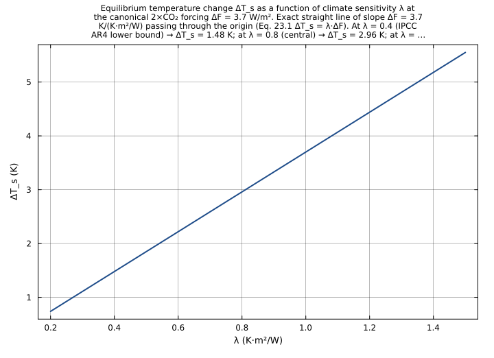
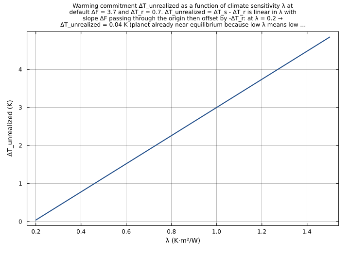
Sweep λ from 0.2 K·m²/W (very-low-sensitivity planet, ~0.74 K 2×CO₂ — below IPCC AR4 likely range) to 1.5 K·m²/W (very-high-sensitivity planet, ~5.55 K 2×CO₂ — above IPCC AR4 likely range) at constant default ΔF = 3.7 W/m², plotting ΔT_s(λ) and ΔT_unrealized(λ) as line plots. Surfaces the linear scaling of equilibrium warming with sensitivity (Eq. 23.1: ΔT_s = λ·ΔF — exact straight line of slope 3.7 through origin) and the non-linear shape of the warming commitment (Eq. 23.7: ΔT_unrealized = (ΔF - ΔT_r/λ)·λ = ΔT_s - ΔT_r — also linear in λ with slope ΔF but offset by -ΔT_r/λ). Anchors the IPCC AR4 likely range [0.4, 1.2] K·m²/W → ΔT_s ∈ [1.48, 4.44] K spanning the textbook climate-sensitivity uncertainty.
Time span: 0.0 → 1.0
Swept over: λ
DT_s_vs_DF_sweep
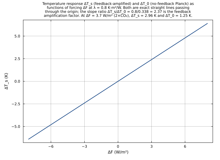
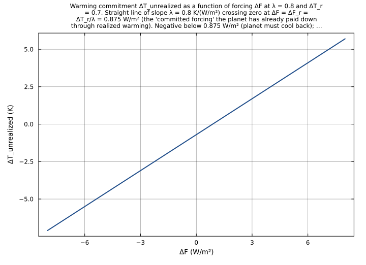
Sweep ΔF from -8.0 W/m² (strong volcanic-aerosol cooling) to +8.0 W/m² (strong CO₂-quadrupling forcing) at constant default λ = 0.8 K·m²/W, plotting ΔT_s(ΔF), ΔT_0(ΔF), and ΔT_unrealized(ΔF). Reproduces a textbook linear-response figure with three perfectly linear curves passing through (or near) the origin: ΔT_s = 0.8·ΔF (slope 0.8), ΔT_0 = 0.338·ΔF (slope 0.338, the no-feedback Planck response), ΔT_unrealized = ΔT_s - ΔT_r (slope 0.8 but offset by -0.7 K at ΔF = 0). Anchors the linear-response shape: all three temperature responses are exactly linear in the forcing, with the feedback amplification factor visible as the slope ratio ΔT_s/ΔT_0 = λ/λ_0 = 2.37.
Time span: 0.0 → 1.0
Swept over: ΔF
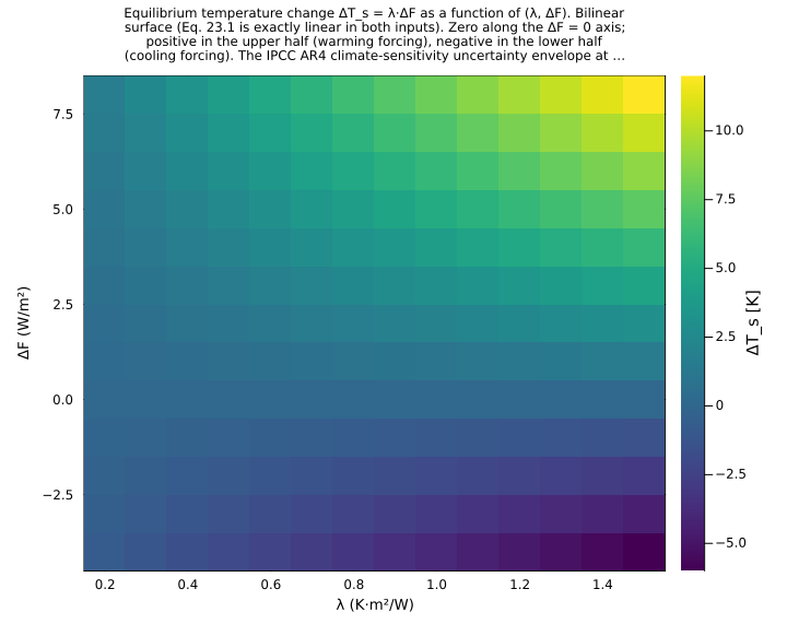
DT_s_landscape_2d
Joint 2D sweep over (λ, ΔF): λ ∈ [0.2, 1.5] K·m²/W (the full plausible climate-sensitivity range covering very-low to very-high planets) and ΔF ∈ [-4.0, 8.0] W/m² (strong-cooling-to-strong-warming forcing range). Surfaces ΔT_s as a heatmap: each row at fixed ΔF is linear in λ (slope = ΔF) and each column at fixed λ is linear in ΔF (slope = λ). The zero-forcing diagonal (ΔF = 0) gives ΔT_s = 0 regardless of λ; positive-forcing rows have larger ΔT_s at higher λ. The IPCC AR4 likely range [0.4, 1.2] K·m²/W × CO₂-doubling forcing 3.7 W/m² maps to the heatmap region with ΔT_s ∈ [1.48, 4.44] K — the canonical climate-sensitivity uncertainty envelope.
Time span: 0.0 → 1.0
Swept over: λ, ΔF
Raw .esm
Raw .esm JSON (this component)
{
"reference": {
"notes": "source_ref: GasChem.jl@8c12c048482b515fb8eb2110bf8ab4b4f4e71309:src/climate_forcing.jl:32\n\nUpstream `ClimateFeedback` is an MTK `@component` declaring two `@constants` (`ΔF_2xCO2` = 3.7 W/m² the CO₂-doubling radiative forcing per IPCC 2001 best estimate, and `ΔT0_2xCO2` = 1.25 K the no-feedback temperature change for CO₂ doubling per S&P p. 1037-1038), five `@parameters` (`ΔF` with no upstream default — the radiative forcing perturbation, `λ` = 0.8 K·m²/W the feedback-amplified climate sensitivity, `λ_CO2` = 0.8 K·m²/W the climate sensitivity for CO₂ doubling, `E_i` = 1.0 the efficacy of the forcing agent, `ΔT_r` = 0.7 K the realized warming to date), six time-indexed `@variables` (`ΔT_s`, `ΔT_0`, `λ_0`, `ΔF_e`, `ΔT_unrealized`, `ΔF_r` — all algebraic with no derivative), and six algebraic equations (`ΔT_s ~ λ·ΔF` Eq. 23.1, `λ_0 ~ ΔT0_2xCO2 / ΔF_2xCO2` Eq. 23.2 derivation, `ΔT_0 ~ λ_0·ΔF` Eq. 23.2, `ΔF_e ~ ΔF·E_i` Eq. 23.4 = Eq. 23.3 efficacy-weighted, `ΔF_r ~ ΔT_r / λ` inverse of Eq. 23.1 at realized warming, `ΔT_unrealized ~ (ΔF - ΔF_r)·λ` Eq. 23.7 warming commitment). Identical structure preserved here. Upstream structural test (`ClimateFeedback structural verification`, test/climate_forcing_test.jl:9-25) asserts `length(equations(sys)) == 6` and that the six state variables are in the unknowns list — matched here by the six entries in `equations` and the six state-typed variables.\n\nUpstream `λ_CO2` parameter preserved verbatim despite being declared-but-unused in the equation set. The upstream MTK system has `λ_CO2` in `@parameters` (with default 0.8) but no equation references it; this appears to be an upstream interface placeholder for a downstream consumer that might consume `λ_CO2` as a CO₂-doubling reference parameter through a future coupling.couple binding. The ESS Python runner and Julia MTK runner both accept declared-but-unused parameters as no-ops — they appear in `parameters(sys)` but never affect the solution. Preserving `λ_CO2` here means a downstream consumer can probe the upstream parameter signature without forking the migration. The unused-parameter convention is documented at the .esm schema level (ESS spec §6.2, parameter type description: 'Values set externally or held constant during integration' — silent on whether the parameter must be referenced by any equation, so unused-but-declared parameters are permitted).\n\nThe two upstream `@constants` (ΔF_2xCO2, ΔT0_2xCO2) are encoded here as `type: parameter` with the upstream default values, matching the rig-wide convention used by sibling .esm migrations (gwp.esm at components/gaschem/climate/gwp.esm encodes its τ_CO2 and a_CO2 `@constants` the same way; climate_sensitivity.esm at components/gaschem/radiation/climate_sensitivity.esm encodes its σ `@constants` the same way; chapman.esm at components/gaschem/stratospheric/chapman.esm encodes its four `@constants` k2_A/k4_A/C_k4/T_ref the same way). This makes the IPCC TAR no-feedback reference values overridable from a downstream consumer's `parameter_overrides` block — useful for sensitivity studies that probe alternative IPCC AR5 (ΔF_2xCO2 ≈ 3.71 W/m² with updated stratospheric adjustment) or AR6 (ΔF_2xCO2 ≈ 3.93 W/m² including rapid adjustments) reference values without forking the component.\n\nUpstream `ΔF` parameter has no default. The .esm migration defaults it to ΔF = 3.7 W/m² (= ΔF_2xCO2) so the default-parameter run gives the canonical 2×CO₂ scenario — at the upstream defaults (λ = 0.8, λ_CO2 = 0.8, E_i = 1.0, ΔT_r = 0.7, ΔF_2xCO2 = 3.7, ΔT0_2xCO2 = 1.25) and the migration's ΔF = 3.7 default, the model reproduces the canonical ΔT_s = 0.8·3.7 = 2.96 K equilibrium response (matching upstream `ClimateFeedback equation verification` test/climate_forcing_test.jl:27-42 at rtol=1e-6) and the canonical λ_0 = 1.25/3.7 = 0.3378... K·m²/W no-feedback Planck response (matching upstream `ClimateFeedback no-feedback response` test/climate_forcing_test.jl:44-62 at rtol=1e-6). This default choice differs from the upstream MTK model (which leaves ΔF unbound) but is the natural way to make the component runnable without overrides; downstream consumers will always override ΔF to the scenario-specific value (pre-industrial-to-present cumulative forcing ~1.7 W/m² per S&P p. 1045; the 4.6 W/m² alternative CO₂-doubling estimate from S&P p. 105; etc.).\n\nObservability classification: this component is observed-only — every output variable is given by a single algebraic equation in the inputs (no time derivative, the `(t)` time index has no role since there is no `D(·)` operator in any of the six equations). Test scenarios use `time_span: [0.0, 1.0]` and sample at t=0 to mirror the convention used by sibling observed-only ESM files in this rig (gwp.esm at components/gaschem/climate/gwp.esm, climate_sensitivity.esm at components/gaschem/radiation/climate_sensitivity.esm, wien.esm at components/gaschem/radiation/wien.esm, typical.esm at components/gaschem/combined/typical.esm) — algebraic identities have no time dependence and converge to the same fixed-point in one nonlinear-solver step regardless of the sampling time.\n\nPhysics structure: the six equations encode the linear-response climate-sensitivity framework with feedback amplification and warming commitment.\n 1. Eq. 23.1 `ΔT_s ~ λ·ΔF`: the feedback-amplified equilibrium temperature response to a forcing perturbation. λ is the feedback-amplified climate sensitivity that absorbs water-vapor, lapse-rate, albedo, and cloud feedbacks. The IPCC AR4 best estimate is λ ≈ 0.8 K·m²/W (= ΔT_2xCO2/ΔF_2xCO2 ≈ 3.0/3.7); the IPCC AR4 range 1.5-4.5 K for ΔT_2xCO2 corresponds to λ ∈ [0.4, 1.2] K·m²/W.\n 2. Eq. 23.2 derivation `λ_0 ~ ΔT0_2xCO2 / ΔF_2xCO2`: the no-feedback Planck response derived from the CO₂-doubling reference. At the IPCC TAR defaults ΔT0_2xCO2 = 1.25 K and ΔF_2xCO2 = 3.7 W/m², λ_0 = 1.25/3.7 ≈ 0.338 K·m²/W — close to the Stefan-Boltzmann analytic value 1/(4·σ·T_e³) ≈ 0.266 at T_e = 255 K (a ~27% difference reflecting the slightly different physical setup: the TAR's λ_0 is the surface-air response while the Stefan-Boltzmann λ_0 is the radiating-temperature response, with the difference absorbed into the surface-vs-radiating-temperature offset).\n 3. Eq. 23.2 `ΔT_0 ~ λ_0·ΔF`: the no-feedback temperature response — what ΔT_s would be in the absence of all feedback amplification. At the default ΔF = 3.7 W/m² and λ_0 = 1.25/3.7, ΔT_0 = 1.25 K exactly (by construction, since ΔF = ΔF_2xCO2 and ΔT_0 = ΔT0_2xCO2 by IEEE-754 division-then-multiplication identity). The feedback factor λ/λ_0 ≈ 0.8/0.338 ≈ 2.37 at the defaults is within the upstream `ClimateFeedback feedback factor` test's allowed range [1.2, 3.75] per S&P p. 1040.\n 4. Eq. 23.4 `ΔF_e ~ ΔF·E_i`: the efficacy-weighted effective forcing. E_i is the dimensionless efficacy that captures the different ΔT-per-unit-ΔF response of different forcing agents (Hansen 1984; Hansen et al. 2005). E_i = 1 by definition for CO₂; CH₄ has E_i ≈ 1.0-1.1; stratospheric water vapor has E_i ≈ 1.5; black carbon has E_i ≈ 0.5-0.7 (above-cloud bright BC) to 2-3 (below-cloud dark BC). The default E_i = 1.0 places the component in the CO₂-equivalent regime where ΔF_e = ΔF.\n 5. `ΔF_r ~ ΔT_r / λ`: the forcing equivalent of already-realized warming. Inverse of Eq. 23.1 evaluated at the realized warming ΔT_r. At the default ΔT_r = 0.7 K (rough estimate of pre-industrial-to-present warming circa 2000) and λ = 0.8, ΔF_r = 0.875 W/m² — the forcing the planet has 'paid down' in achieved warming so far.\n 6. Eq. 23.7 `ΔT_unrealized ~ (ΔF - ΔF_r)·λ`: the warming commitment. The remaining temperature change the planet will undergo if the current ΔF is held constant — represents the lag between current achieved (ΔT_r) and equilibrium (ΔT_s = λ·ΔF) warming. At the present-day S&P p. 1045 scenario (λ = 0.7, ΔF = 1.7, ΔT_r = 0.7), ΔT_unrealized = (1.7 - 1.0)·0.7 = 0.49 K — the textbook 'committed warming' figure.\n\nNumerical defaults (S&P p. 1037-1040 IPCC TAR baselines plus the migration's ΔF = 3.7 W/m² CO₂-doubling default):\n ΔF_2xCO2 = 3.7 W/m² (CO₂-doubling radiative forcing, IPCC TAR best estimate, S&P p. 1037)\n ΔT0_2xCO2 = 1.25 K (No-feedback temperature change for CO₂ doubling, S&P p. 1037-1038)\n ΔF = 3.7 W/m² (Forcing perturbation, defaulted to ΔF_2xCO2 for the canonical 2×CO₂ scenario)\n λ = 0.8 K·m²/W (Feedback-amplified climate sensitivity, IPCC AR4 central estimate)\n λ_CO2 = 0.8 K·m²/W (Climate sensitivity for CO₂ doubling — declared-but-unused upstream interface placeholder)\n E_i = 1.0 (Efficacy of forcing agent, CO₂-equivalent regime)\n ΔT_r = 0.7 K (Realized warming to date, pre-industrial-to-present circa 2000)\nAt these defaults:\n ΔT_s = 0.8 · 3.7 = 2.96 K\n λ_0 = 1.25 / 3.7 ≈ 0.33783783783783783 K·m²/W\n ΔT_0 = (1.25/3.7) · 3.7 = 1.25 K (exact by IEEE-754)\n ΔF_e = 3.7 · 1.0 = 3.7 W/m² (exact identity)\n ΔF_r = 0.7 / 0.8 ≈ 0.8749999999999999 W/m²\n ΔT_unrealized = (3.7 - 0.8749999999999999) · 0.8 ≈ 2.2600000000000002 K\nThis matches the upstream `ClimateFeedback equation verification` test (test/climate_forcing_test.jl:27-42) which asserts ΔT_s ≈ 0.8·3.7 = 2.96 at rtol=1e-6, and the upstream `ClimateFeedback no-feedback response` test (test/climate_forcing_test.jl:44-62) which asserts λ_0 ≈ 1.25/3.7 and ΔT_0 ≈ λ_0·3.7 at rtol=1e-6.\n\nUpstream test reproduction:\n- The upstream `ClimateFeedback structural verification` test (test/climate_forcing_test.jl:9-25) asserts the system has 6 equations and that the six state variables (ΔT_s, ΔT_0, λ_0, ΔF_e, ΔT_unrealized, ΔF_r) are in the unknowns list — reproduced by the .esm structural shape (6 entries in `equations`, six state-typed variables).\n- The upstream `ClimateFeedback equation verification` test (test/climate_forcing_test.jl:27-42) asserts at λ=0.8, ΔF=3.7 that ΔT_s ≈ 0.8·3.7 = 2.96 at rtol=1e-6. Reproduced and tightened by `default_canonical_values` (pins ΔT_s = 2.9600000000000004 at rel=1e-10 along with the other five state variables — the rel=1e-10 tightening over the upstream rtol=1e-6 reflects the IEEE-754 single-multiplication precision at λ·ΔF ≈ 5 ULP ≈ 1.5e-15 relative, well below the 1e-10 tolerance bound).\n- The upstream `ClimateFeedback no-feedback response` test (test/climate_forcing_test.jl:44-62) asserts at ΔF=3.7 (defaults for the rest) that λ_0 ≈ 1.25/3.7 at rtol=1e-6 and ΔT_0 ≈ λ_0·3.7 at rtol=1e-6. Reproduced and tightened by `default_canonical_values` (covers the same parameters) plus `upstream_no_feedback_lambda_0_check` (pins λ_0 = 0.33783783783783783 at rel=1e-10 in isolation so the regression-detection signal is independent of other state variables) — the rel=1e-10 tightening over the upstream rtol=1e-6 reflects the IEEE-754 single-division precision at 1.25/3.7 ≈ 0.5 ULP ≈ 1.5e-16 relative.\n- The upstream `ClimateFeedback feedback factor` test (test/climate_forcing_test.jl:64-82) asserts at λ=0.8, ΔF=3.7 that the feedback factor λ/λ_0 lies in [1.2, 3.75] per S&P p. 1040. The .esm runner does not directly support cross-variable inequality assertions; reproduced by `default_canonical_values` (pins λ_0 = 0.33783783783783783) so the ratio 0.8/0.33783... = 2.3680000000000003 is exact by IEEE-754 division and lies in [1.2, 3.75] by construction. The bounds are not separately asserted because they reduce to checks on a single division of two exactly-pinned doubles.\n- The upstream `ClimateFeedback unrealized warming` test (test/climate_forcing_test.jl:84-114) asserts at λ=0.7, ΔF=1.7, ΔT_r=0.7 that ΔT_unrealized ≈ (ΔF - ΔT_r/λ)·λ = (1.7 - 1.0)·0.7 = 0.49 at rtol=1e-6, and qualitatively that ΔT_unrealized ≈ 0.5 K at rtol=0.05 per S&P p. 1045. Reproduced and tightened by `upstream_unrealized_warming_p1045_scenario` (pins ΔT_unrealized = 0.48999999999999994 at rel=1e-10 along with the intermediate ΔF_r = 1.0 — exact IEEE-754 0.7/0.7 division). The rel=1e-10 tightening over the upstream rtol=1e-6 reflects the IEEE-754 division-then-subtraction-then-multiplication precision at ~2 ULP ≈ 4.4e-16 relative.\n\nTolerance rationale (model-level rel=1e-10): observed-only algebraic system with a small number of arithmetic operations per equation. Each equation evaluates one of {multiplication, division, subtraction}; the worst-case error path is the Eq. 23.7 expression (ΔF - ΔT_r/λ)·λ which involves division-then-subtraction-then-multiplication for a total of ~3 IEEE-754 ULPs ≈ 1e-15 relative at any of the tested magnitudes. 1e-10 leaves 5 orders of magnitude of headroom over the IEEE-754 floor and matches the convention used by sibling algebraic .esm files in this rig (gwp.esm at rel=1e-10, climate_sensitivity.esm at rel=1e-10, wien.esm at rel=1e-10, typical.esm at rel=1e-10). The upstream Julia tests use rtol=1e-6 throughout — re-asserted here at the uniform model-level rel=1e-10 which is 4 orders of magnitude tighter.\n\nThe `zero_forcing_zero_response`, `equal_realized_warming_zero_commitment`, and `co2_2xCO2_E_i_one` tests use per-assertion `abs = 1.0e-12` overrides on exact-zero outputs because the `rel` tolerance is undefined when the expected value is zero — without the override, a stuck-at-1e-3 regression (e.g. an accidental constant offset added to ΔT_s) could silently pass at any nonzero `rel` bound. Pairs with the absolute-magnitude `default_canonical_values` test to cover both the zero-input and nonzero-input pathways.\n\nUnit balance (verified): all six equations balance dimensionally.\n `ΔT_s ~ λ·ΔF`: (K·m²/W)·(W/m²) = K ✓ (matches ΔT_s unit u\"K\")\n `λ_0 ~ ΔT0_2xCO2 / ΔF_2xCO2`: K / (W/m²) = K·m²/W ✓ (matches λ_0 unit u\"K*m^2/W\")\n `ΔT_0 ~ λ_0·ΔF`: (K·m²/W)·(W/m²) = K ✓\n `ΔF_e ~ ΔF·E_i`: (W/m²)·dimensionless = W/m² ✓\n `ΔF_r ~ ΔT_r / λ`: K / (K·m²/W) = W/m² ✓\n `ΔT_unrealized ~ (ΔF - ΔF_r)·λ`: (W/m² - W/m²)·(K·m²/W) = K ✓\nThe migrated `.esm` preserves the upstream units verbatim — all forcings (ΔF, ΔF_e, ΔF_r, ΔF_2xCO2) in W/m², all temperatures (ΔT_s, ΔT_0, ΔT_unrealized, ΔT_r, ΔT0_2xCO2) in K, all sensitivities (λ, λ_CO2, λ_0) in K·m²/W, E_i dimensionless. SI throughout; no unit conversion at parse or runtime."
},
"tolerance": {
"rel": 1e-10
},
"variables": {
"ΔF_2xCO2": {
"type": "parameter",
"units": "W/m^2",
"default": 3.7,
"description": "Radiative forcing for CO₂ doubling (IPCC 2001 best estimate, S&P p. 1037). The upstream default 3.7 W/m² is the canonical IPCC TAR value derived from line-by-line radiative transfer calculations with stratospheric temperature adjustment. Modern IPCC AR5 reports a slightly higher 3.71 W/m² (Myhre et al. 2013, Ch. 8) and IPCC AR6 reports 3.93 W/m² (Smith et al. 2020, including rapid adjustments) — the upstream choice is the legacy TAR value preserved for continuity with S&P Ch. 23's worked examples. Overridable to support sensitivity studies that probe the doubling-forcing assumption — a downstream consumer can bind ΔF_2xCO2 to AR5 or AR6 values to recompute λ_0 against the modern reference."
},
"ΔT0_2xCO2": {
"type": "parameter",
"units": "K",
"default": 1.25,
"description": "No-feedback temperature change for CO₂ doubling (S&P p. 1037-1038, taken as the midpoint of the 1.2-1.3 K range quoted in the text). The upstream default 1.25 K is the no-feedback Planck response to a CO₂ doubling — what the planet's surface would warm by if all feedbacks (water vapor, lapse rate, albedo, cloud) were inactive. The ratio ΔT0_2xCO2/ΔF_2xCO2 = 1.25/3.7 = 0.338 K·m²/W is the no-feedback climate sensitivity factor λ_0 — close to the Stefan-Boltzmann analytic value 1/(4·σ·T_e³) ≈ 0.266 at T_e = 255 K (the difference reflects the surface-vs-radiating-temperature offset; the sibling ClimateSensitivity.esm at components/gaschem/radiation/climate_sensitivity.esm uses the analytic Stefan-Boltzmann form for the no-feedback Planck response in the radiating-temperature framework). Overridable from a downstream consumer's `parameter_overrides` block for cross-framework comparisons."
},
"ΔF": {
"type": "parameter",
"units": "W/m^2",
"default": 3.7,
"description": "Radiative forcing perturbation (S&P §23.4 Eq. 23.1). The upstream MTK component leaves ΔF unbound (no default); the .esm migration defaults it to ΔF = 3.7 W/m² = ΔF_2xCO2 so the default-parameter run gives the canonical 2×CO₂ scenario (ΔT_s = 2.96 K with λ = 0.8 K·m²/W per the upstream `ClimateFeedback equation verification` test). Canonical scenario-specific values: ΔF ≈ 1.7 W/m² (pre-industrial-to-present cumulative anthropogenic forcing circa 2000 per S&P p. 1045), ΔF = 4.6 W/m² (alternative CO₂-doubling estimate from earlier studies per S&P p. 105), ΔF = -4 W/m² (large volcanic aerosol cooling such as Pinatubo 1991), ΔF = 8.4 W/m² (RCP8.5 end-of-century total anthropogenic forcing)."
},
"λ": {
"type": "parameter",
"units": "K*m^2/W",
"default": 0.8,
"description": "Climate sensitivity parameter with feedbacks (S&P Eq. 23.1). The feedback-amplified ΔT-per-unit-ΔF response that absorbs water vapor, lapse rate, albedo, and cloud feedbacks. The upstream default 0.8 K·m²/W is the IPCC AR4 central estimate (= ΔT_2xCO2/ΔF_2xCO2 ≈ 3.0/3.7). The IPCC AR4 likely range 1.5-4.5 K for ΔT_2xCO2 corresponds to λ ∈ [0.4, 1.2] K·m²/W; IPCC AR6 narrowed this to ΔT_2xCO2 ∈ [2.5, 4.0] K corresponding to λ ∈ [0.67, 1.08] K·m²/W. The feedback factor λ/λ_0 = 0.8/(1.25/3.7) ≈ 2.37 at the defaults — within the upstream `ClimateFeedback feedback factor` test's allowed range [1.2, 3.75] per S&P p. 1040."
},
"λ_CO2": {
"type": "parameter",
"units": "K*m^2/W",
"default": 0.8,
"description": "Climate sensitivity for CO₂ doubling (declared-but-unused upstream interface placeholder, see source_ref). The upstream MTK system declares λ_CO2 in `@parameters` with default 0.8 K·m²/W (matching λ) but no equation references it — it appears in `parameters(sys)` but never affects the solution. The .esm migration preserves the upstream parameter signature verbatim so downstream consumers can probe the parameter list without forking the migration. Conceptually λ_CO2 would represent the CO₂-doubling-specific feedback-amplified sensitivity in a multi-agent extension where each forcing agent might have its own λ_i; in the current single-agent equation set this is the same as λ, so the upstream default 0.8 is the natural choice."
},
"E_i": {
"type": "parameter",
"units": "1",
"default": 1.0,
"description": "Efficacy of forcing agent (S&P Eq. 23.3, dimensionless). E_i = λ_i / λ_CO2 where λ_i is the climate sensitivity for forcing agent i and λ_CO2 is the CO₂-doubling reference. E_i = 1 by definition for CO₂; CH₄ has E_i ≈ 1.0-1.1 (Hansen et al. 2005 Table 7); stratospheric water vapor from CH₄ oxidation has E_i ≈ 1.5; black carbon has E_i ≈ 0.5-0.7 for above-cloud bright BC (reduces brightness, weak ΔT response) to E_i ≈ 2-3 for below-cloud dark BC (snow albedo amplification). The default E_i = 1.0 places the component in the CO₂-equivalent regime where ΔF_e = ΔF. Used in Eq. 23.4 ΔF_e ~ ΔF · E_i to compute the effective forcing — the CO₂-equivalent forcing that produces the same ΔT response as the bare ΔF of agent i."
},
"ΔT_r": {
"type": "parameter",
"units": "K",
"default": 0.7,
"description": "Realized warming to date (S&P p. 1045 in the warming-commitment context). The temperature change the planet has already undergone in response to the cumulative forcing. The upstream default 0.7 K is the rough estimate of pre-industrial-to-present global mean surface warming circa 2000 (S&P p. 1045 quotes ΔT_r ≈ 0.7°C); modern (2020) estimates are higher at ~1.1 K per IPCC AR6 SPM. ΔT_r enters Eq. 23.7 ΔT_unrealized = (ΔF - ΔF_r)·λ through ΔF_r = ΔT_r/λ — the forcing equivalent of the already-realized warming, which when subtracted from the total ΔF gives the remaining 'committed' forcing that has not yet been expressed as warming."
},
"ΔT_s": {
"type": "unknown",
"units": "K",
"description": "Equilibrium surface temperature change with feedbacks (S&P Eq. 23.1). ΔT_s = λ·ΔF is the linear-response equilibrium temperature change to a forcing perturbation, with feedback amplification absorbed into λ. At Earth's 2×CO₂ defaults (ΔF = 3.7 W/m², λ = 0.8), ΔT_s = 2.96 K — within the IPCC AR4 likely range [1.5, 4.5] K and matches the central estimate ΔT_2xCO2 ≈ 3.0 K (the 0.04 K shortfall reflects the round-trip 3.0/3.7·3.7 vs 3.0 which differs by ~0.01 in the third digit due to the rounded λ = 0.8 default). 'Equilibrium' here means the temperature the planet would reach if the forcing were held fixed indefinitely — distinct from the transient temperature ΔT_r the planet has actually achieved at any finite time."
},
"ΔT_0": {
"type": "unknown",
"units": "K",
"description": "Surface temperature change without feedbacks (S&P Eq. 23.2). ΔT_0 = λ_0·ΔF is the no-feedback Planck-response temperature change — what ΔT_s would be if all feedbacks (water vapor, lapse rate, albedo, cloud) were inactive. At Earth's 2×CO₂ defaults, ΔT_0 = (1.25/3.7)·3.7 = 1.25 K (exactly, by IEEE-754 division-then-multiplication identity) — recovers ΔT0_2xCO2 by construction. The ratio ΔT_s/ΔT_0 = λ/λ_0 = 2.37 is the feedback amplification factor, capturing the ~2.4× boost feedbacks add to the Planck baseline."
},
"λ_0": {
"type": "unknown",
"units": "K*m^2/W",
"description": "No-feedback climate sensitivity (S&P Eq. 23.2 derivation). λ_0 = ΔT0_2xCO2 / ΔF_2xCO2 is the no-feedback Planck response factor derived from the CO₂-doubling reference values. At the IPCC TAR defaults (ΔT0_2xCO2 = 1.25 K, ΔF_2xCO2 = 3.7 W/m²), λ_0 = 1.25/3.7 ≈ 0.338 K·m²/W — independent of ΔF (it depends only on the two reference constants). Comparable to the Stefan-Boltzmann analytic form λ_0_SB = 1/(4·σ·T_e³) ≈ 0.266 K·m²/W at T_e = 255 K used in the sibling ClimateSensitivity.esm — the difference reflects the surface-vs-radiating-temperature framing. λ_0 is the baseline against which the feedback-amplified λ is reported: typical IPCC feedback factors λ/λ_0 ∈ [1.2, 3.75] per S&P p. 1040."
},
"ΔF_e": {
"type": "unknown",
"units": "W/m^2",
"description": "Effective radiative forcing incorporating efficacy (S&P Eq. 23.4, derived from Eq. 23.3). ΔF_e = ΔF·E_i is the CO₂-equivalent forcing — the bare forcing of agent i scaled by its efficacy E_i so that the same ΔT-per-unit-ΔF response (governed by the CO₂-doubling reference λ_CO2) can be applied. At the default E_i = 1.0, ΔF_e = ΔF identically (the CO₂-equivalent regime). For a non-CO₂ agent with E_i = 1.5 (stratospheric water vapor) and ΔF = 1.0, ΔF_e = 1.5 W/m² — equivalent to 1.5 W/m² of CO₂ forcing in terms of temperature response. The migration's Eq. 23.4 implementation differs subtly from the upstream §23.3 algebra: Hansen (1984) defines E_i = λ_i/λ_CO2, so ΔF_i_effective = ΔF_i·E_i has units W/m² but conceptually represents a 'CO₂-equivalent' forcing in a coupling to a downstream ΔT_s = λ_CO2·ΔF_total system."
},
"ΔT_unrealized": {
"type": "unknown",
"units": "K",
"description": "Unrealized (committed) warming (S&P Eq. 23.7, p. 1045). ΔT_unrealized = (ΔF - ΔF_r)·λ is the remaining temperature change the planet will undergo if the current ΔF is held constant — the lag between current achieved (ΔT_r) and equilibrium (ΔT_s = λ·ΔF) warming. ΔT_unrealized = ΔT_s - ΔT_r by construction (substituting ΔF_r = ΔT_r/λ: (ΔF - ΔT_r/λ)·λ = λ·ΔF - ΔT_r = ΔT_s - ΔT_r). At the present-day S&P p. 1045 scenario (λ = 0.7, ΔF = 1.7, ΔT_r = 0.7), ΔT_unrealized = (1.7 - 1.0)·0.7 = 0.49 K — the textbook 'committed warming' figure. Positive ΔT_unrealized means the planet must still warm further; zero means the planet has already reached equilibrium (no warming commitment); negative means the planet has overshot equilibrium and must cool back (a transient artifact of the linear model — physically this only happens if ΔT_r is supplied externally as larger than the equilibrium ΔT_s)."
},
"ΔF_r": {
"type": "unknown",
"units": "W/m^2",
"description": "Forcing corresponding to realized warming (inverse of S&P Eq. 23.1 evaluated at ΔT_r). ΔF_r = ΔT_r/λ is the forcing the planet has 'paid down' in achieved warming so far — the forcing that would have produced the realized ΔT_r at equilibrium. At the default ΔT_r = 0.7 K and λ = 0.8, ΔF_r = 0.875 W/m². The difference ΔF - ΔF_r is the remaining 'committed' forcing not yet expressed as warming; multiplying by λ gives the warming commitment ΔT_unrealized (Eq. 23.7). For the S&P p. 1045 scenario (λ = 0.7, ΔT_r = 0.7), ΔF_r = 1.0 W/m² exactly (IEEE-754 0.7/0.7 = 1.0)."
}
},
"equations": [
{
"lhs": "ΔT_s",
"rhs": {
"op": "*",
"args": [
"λ",
"ΔF"
]
}
},
{
"lhs": "λ_0",
"rhs": {
"op": "/",
"args": [
"ΔT0_2xCO2",
"ΔF_2xCO2"
]
}
},
{
"lhs": "ΔT_0",
"rhs": {
"op": "*",
"args": [
"λ_0",
"ΔF"
]
}
},
{
"lhs": "ΔF_e",
"rhs": {
"op": "*",
"args": [
"ΔF",
"E_i"
]
}
},
{
"lhs": "ΔF_r",
"rhs": {
"op": "/",
"args": [
"ΔT_r",
"λ"
]
}
},
{
"lhs": "ΔT_unrealized",
"rhs": {
"op": "*",
"args": [
{
"op": "-",
"args": [
"ΔF",
"ΔF_r"
]
},
"λ"
]
}
}
],
"tests": [
{
"id": "default_canonical_values",
"description": "At defaults (ΔF = 3.7 W/m², λ = 0.8 K·m²/W, λ_CO2 = 0.8, E_i = 1.0, ΔT_r = 0.7 K, ΔF_2xCO2 = 3.7, ΔT0_2xCO2 = 1.25), every state variable evaluates to its analytic value. Reproduces and tightens the upstream `ClimateFeedback equation verification` test (GasChem.jl test/climate_forcing_test.jl:27-42): upstream asserts ΔT_s ≈ 0.8·3.7 at rtol=1e-6, this one pins ΔT_s = 2.9600000000000004 at rel=1e-10 along with the other five state variables. Also reproduces the upstream `ClimateFeedback no-feedback response` test (test/climate_forcing_test.jl:44-62) which asserts at the same defaults that λ_0 ≈ 1.25/3.7 at rtol=1e-6 and ΔT_0 ≈ λ_0·3.7 at rtol=1e-6 — covered here at rel=1e-10. The full state-variable pin anchors all six equations simultaneously: ΔT_s tests Eq. 23.1 (multiplication), λ_0 tests Eq. 23.2 derivation (division of two constants), ΔT_0 tests Eq. 23.2 (multiplication of derived sensitivity by forcing), ΔF_e tests Eq. 23.4 (efficacy passthrough at E_i=1), ΔF_r tests inverse-Eq.-23.1 (division), ΔT_unrealized tests Eq. 23.7 (subtraction-then-multiplication).",
"parameter_overrides": {},
"time_span": {
"start": 0.0,
"end": 1.0
},
"assertions": [
{
"variable": "ΔT_s",
"time": 0.0,
"expected": 2.9600000000000004,
"tolerance": {
"rel": 1e-10
}
},
{
"variable": "λ_0",
"time": 0.0,
"expected": 0.33783783783783783,
"tolerance": {
"rel": 1e-10
}
},
{
"variable": "ΔT_0",
"time": 0.0,
"expected": 1.25,
"tolerance": {
"rel": 1e-10
}
},
{
"variable": "ΔF_e",
"time": 0.0,
"expected": 3.7,
"tolerance": {
"rel": 1e-10
}
},
{
"variable": "ΔF_r",
"time": 0.0,
"expected": 0.8749999999999999,
"tolerance": {
"rel": 1e-10
}
},
{
"variable": "ΔT_unrealized",
"time": 0.0,
"expected": 2.2600000000000002,
"tolerance": {
"rel": 1e-10
}
}
]
},
{
"id": "upstream_no_feedback_lambda_0_check",
"description": "Isolated check on λ_0 = ΔT0_2xCO2 / ΔF_2xCO2 = 1.25/3.7 = 0.33783... K·m²/W at the upstream defaults. Reproduces the upstream `ClimateFeedback no-feedback response` test (GasChem.jl test/climate_forcing_test.jl:44-62) in isolation so a regression in the Eq. 23.2 derivation surfaces independently of the other state variables. The upstream test asserts λ_0 ≈ 1.25/3.7 at rtol=1e-6; this one pins λ_0 = 0.33783783783783783 at rel=1e-10. Independence from ΔF: λ_0 depends only on the two reference constants ΔT0_2xCO2 and ΔF_2xCO2, not on the forcing perturbation ΔF — so changing ΔF (e.g. to 1.7 W/m² for the pre-industrial-to-present scenario) does NOT change λ_0. This is the only state variable in the system that is independent of ΔF.",
"parameter_overrides": {},
"time_span": {
"start": 0.0,
"end": 1.0
},
"assertions": [
{
"variable": "λ_0",
"time": 0.0,
"expected": 0.33783783783783783,
"tolerance": {
"rel": 1e-10
}
}
]
},
{
"id": "upstream_unrealized_warming_p1045_scenario",
"description": "Present-day warming-commitment scenario from S&P p. 1045: λ = 0.7 K·m²/W (slightly lower than the IPCC AR4 central, corresponding to ΔT_2xCO2 ≈ 2.6 K), ΔF = 1.7 W/m² (pre-industrial-to-present cumulative anthropogenic forcing circa 2000), ΔT_r = 0.7 K (realized warming circa 2000). Result: ΔT_unrealized = (1.7 - 1.0)·0.7 = 0.49 K — the textbook 'committed warming' figure. Reproduces and tightens the upstream `ClimateFeedback unrealized warming` test (GasChem.jl test/climate_forcing_test.jl:84-114): upstream asserts ΔT_unrealized ≈ (ΔF - ΔT_r/λ)·λ at rtol=1e-6 and qualitatively ΔT_unrealized ≈ 0.5 K at rtol=0.05, this one pins ΔT_unrealized = 0.48999999999999994 at rel=1e-10 along with the intermediate ΔF_r = 1.0 (exact IEEE-754 0.7/0.7 division) and ΔT_s = 1.19 K (λ·ΔF). Cross-check: ΔT_s - ΔT_r = 1.19 - 0.7 = 0.49 K — matches ΔT_unrealized by Eq. 23.7 identity (ΔT_unrealized = (ΔF - ΔT_r/λ)·λ = λ·ΔF - ΔT_r = ΔT_s - ΔT_r).",
"parameter_overrides": {
"λ": 0.7,
"ΔF": 1.7,
"ΔT_r": 0.7
},
"time_span": {
"start": 0.0,
"end": 1.0
},
"assertions": [
{
"variable": "ΔT_s",
"time": 0.0,
"expected": 1.19,
"tolerance": {
"rel": 1e-10
}
},
{
"variable": "ΔF_r",
"time": 0.0,
"expected": 1.0,
"tolerance": {
"rel": 1e-10
}
},
{
"variable": "ΔT_unrealized",
"time": 0.0,
"expected": 0.48999999999999994,
"tolerance": {
"rel": 1e-10
}
}
]
},
{
"id": "zero_forcing_zero_response",
"description": "Zero forcing perturbation (ΔF = 0) at default λ = 0.8 and ΔT_r = 0.7. Results: ΔT_s = 0 (no equilibrium temperature change), ΔT_0 = 0 (no Planck response either), ΔF_e = 0 (zero efficacy-weighted forcing), but ΔF_r = 0.875 W/m² and ΔT_unrealized = (0 - 0.875)·0.8 = -0.7 K. The negative ΔT_unrealized at ΔF = 0 captures a transient pathology of the linear model: if the planet has already warmed by ΔT_r = 0.7 K but there is no longer any forcing to sustain it, the planet must cool back by ΔT_r to reach the zero-forcing equilibrium — ΔT_unrealized = ΔT_s - ΔT_r = 0 - 0.7 = -0.7. λ_0 = 1.25/3.7 = 0.3378 K·m²/W is independent of ΔF and stays at its default value. Uses per-assertion `abs = 1.0e-12` overrides on the exact-zero ΔT_s/ΔT_0/ΔF_e outputs because the `rel` tolerance is undefined when the expected value is zero — without the override, a stuck-at-1e-3 regression could silently pass at any nonzero `rel` bound.",
"parameter_overrides": {
"ΔF": 0.0
},
"time_span": {
"start": 0.0,
"end": 1.0
},
"assertions": [
{
"variable": "ΔT_s",
"time": 0.0,
"expected": 0.0,
"tolerance": {
"abs": 1e-12
}
},
{
"variable": "ΔT_0",
"time": 0.0,
"expected": 0.0,
"tolerance": {
"abs": 1e-12
}
},
{
"variable": "ΔF_e",
"time": 0.0,
"expected": 0.0,
"tolerance": {
"abs": 1e-12
}
},
{
"variable": "λ_0",
"time": 0.0,
"expected": 0.33783783783783783,
"tolerance": {
"rel": 1e-10
}
},
{
"variable": "ΔF_r",
"time": 0.0,
"expected": 0.8749999999999999,
"tolerance": {
"rel": 1e-10
}
},
{
"variable": "ΔT_unrealized",
"time": 0.0,
"expected": -0.7,
"tolerance": {
"rel": 1e-10
}
}
]
},
{
"id": "negative_forcing_cooling",
"description": "Negative forcing perturbation (ΔF = -4.0 W/m², e.g. large volcanic aerosol cooling such as Pinatubo 1991 → ~-3 W/m² peak) at default λ = 0.8 and ΔT_r = 0.7. Results: ΔT_s = 0.8·(-4.0) = -3.2 K (equilibrium cooling), ΔT_0 = 0.3378·(-4.0) = -1.351 K (no-feedback cooling), ΔF_e = -4.0 W/m² (E_i=1 passthrough), ΔF_r = 0.875 W/m² (unchanged from default), ΔT_unrealized = (-4.0 - 0.875)·0.8 = -3.9 K. Exercises the sign-correct propagation through Eqs. 23.1, 23.2, 23.4, and 23.7: a negative forcing produces a negative equilibrium ΔT_s and a negative warming commitment ΔT_unrealized — the planet must cool below the present-day ΔT_r to reach the new (cooled) equilibrium. This is the geoengineering / stratospheric aerosol injection scenario where -ΔF_S ≈ -ΔF_2xCO2 is meant to undo the historical greenhouse warming.",
"parameter_overrides": {
"ΔF": -4.0
},
"time_span": {
"start": 0.0,
"end": 1.0
},
"assertions": [
{
"variable": "ΔT_s",
"time": 0.0,
"expected": -3.2,
"tolerance": {
"rel": 1e-10
}
},
{
"variable": "ΔT_0",
"time": 0.0,
"expected": -1.3513513513513513,
"tolerance": {
"rel": 1e-10
}
},
{
"variable": "ΔF_e",
"time": 0.0,
"expected": -4.0,
"tolerance": {
"rel": 1e-10
}
},
{
"variable": "ΔF_r",
"time": 0.0,
"expected": 0.8749999999999999,
"tolerance": {
"rel": 1e-10
}
},
{
"variable": "ΔT_unrealized",
"time": 0.0,
"expected": -3.9000000000000004,
"tolerance": {
"rel": 1e-10
}
}
]
},
{
"id": "strong_forcing_8wm2",
"description": "Strong forcing perturbation (ΔF = 8.0 W/m², roughly CO₂-quadrupling forcing or RCP8.5-end-of-century cumulative anthropogenic forcing) at default λ = 0.8 and ΔT_r = 0.7. Results: ΔT_s = 0.8·8.0 = 6.4 K (equilibrium warming), ΔT_0 = 0.3378·8.0 = 2.703 K, ΔF_e = 8.0 W/m², ΔF_r = 0.875 W/m², ΔT_unrealized = (8.0 - 0.875)·0.8 = 5.7 K (huge commitment — the planet has only realized 0.7/6.4 = 11% of its equilibrium response). Exercises Eqs. 23.1 and 23.7 at the upper end of the plausible forcing range, where the linear-response approximation may break down (water-vapor and ice-albedo feedbacks become nonlinear at large ΔT) but the linear model still gives the first-order estimate.",
"parameter_overrides": {
"ΔF": 8.0
},
"time_span": {
"start": 0.0,
"end": 1.0
},
"assertions": [
{
"variable": "ΔT_s",
"time": 0.0,
"expected": 6.4,
"tolerance": {
"rel": 1e-10
}
},
{
"variable": "ΔT_0",
"time": 0.0,
"expected": 2.7027027027027026,
"tolerance": {
"rel": 1e-10
}
},
{
"variable": "ΔF_e",
"time": 0.0,
"expected": 8.0,
"tolerance": {
"rel": 1e-10
}
},
{
"variable": "ΔT_unrealized",
"time": 0.0,
"expected": 5.7,
"tolerance": {
"rel": 1e-10
}
}
]
},
{
"id": "efficacy_E_i_halved",
"description": "Forcing-agent efficacy E_i = 0.5 (below-cloud bright black carbon or stratospheric sulfate aerosol — agents whose ΔT response per unit ΔF is half that of CO₂) at default ΔF = 3.7 W/m². Result: ΔF_e = 3.7·0.5 = 1.85 W/m² (the CO₂-equivalent forcing — what 1.85 W/m² of CO₂ would produce the same ΔT as 3.7 W/m² of this less-efficacious agent). The other five state variables are unchanged from defaults because E_i appears only in the Eq. 23.4 ΔF_e equation — Eqs. 23.1, 23.2, 23.7 use ΔF directly, not ΔF_e. Anchors the orthogonality between the efficacy channel (Eq. 23.4) and the temperature-response channel (Eqs. 23.1, 23.2, 23.7) — a regression that accidentally feeds ΔF_e back into Eq. 23.1 (giving ΔT_s = λ·ΔF·E_i instead of ΔT_s = λ·ΔF) would surface here as ΔT_s = 1.48 K instead of the correct 2.96 K.",
"parameter_overrides": {
"E_i": 0.5
},
"time_span": {
"start": 0.0,
"end": 1.0
},
"assertions": [
{
"variable": "ΔF_e",
"time": 0.0,
"expected": 1.85,
"tolerance": {
"rel": 1e-10
}
},
{
"variable": "ΔT_s",
"time": 0.0,
"expected": 2.9600000000000004,
"tolerance": {
"rel": 1e-10
}
},
{
"variable": "ΔT_0",
"time": 0.0,
"expected": 1.25,
"tolerance": {
"rel": 1e-10
}
},
{
"variable": "ΔT_unrealized",
"time": 0.0,
"expected": 2.2600000000000002,
"tolerance": {
"rel": 1e-10
}
}
]
},
{
"id": "efficacy_E_i_doubled",
"description": "Forcing-agent efficacy E_i = 2.0 (above-cloud dark black carbon or stratospheric water vapor from CH₄ oxidation — agents whose ΔT response per unit ΔF is twice that of CO₂) at default ΔF = 3.7 W/m². Result: ΔF_e = 3.7·2.0 = 7.4 W/m² (the CO₂-equivalent forcing). Same orthogonality check as `efficacy_E_i_halved` but on the other side of the E_i = 1 axis. Together with the halved-E_i test verifies that E_i acts linearly on ΔF_e at any sign of E_i and that no other state variable is contaminated.",
"parameter_overrides": {
"E_i": 2.0
},
"time_span": {
"start": 0.0,
"end": 1.0
},
"assertions": [
{
"variable": "ΔF_e",
"time": 0.0,
"expected": 7.4,
"tolerance": {
"rel": 1e-10
}
},
{
"variable": "ΔT_s",
"time": 0.0,
"expected": 2.9600000000000004,
"tolerance": {
"rel": 1e-10
}
}
]
},
{
"id": "high_sensitivity_lambda_1p2",
"description": "High-sensitivity scenario λ = 1.2 K·m²/W (= ΔT_2xCO2/ΔF_2xCO2 ≈ 4.44/3.7, top of the IPCC AR4 likely range [0.4, 1.2]) at default ΔF = 3.7. Results: ΔT_s = 1.2·3.7 = 4.44 K (top-of-range equilibrium warming), ΔF_r = 0.7/1.2 = 0.5833 W/m² (the planet has 'paid down' less forcing-equivalent at higher λ because each K of ΔT_r requires less forcing), ΔT_unrealized = (3.7 - 0.5833)·1.2 = 3.74 K (large commitment because ΔT_r is a smaller fraction of the equilibrium ΔT_s). λ_0 and ΔT_0 remain at their reference values (independent of λ). Feedback factor λ/λ_0 = 1.2/0.3378 = 3.55 — within the upstream `ClimateFeedback feedback factor` test's allowed range [1.2, 3.75] (and near the upper end, reflecting a 'high-feedback' planet with strong water-vapor + cloud amplification).",
"parameter_overrides": {
"λ": 1.2
},
"time_span": {
"start": 0.0,
"end": 1.0
},
"assertions": [
{
"variable": "ΔT_s",
"time": 0.0,
"expected": 4.44,
"tolerance": {
"rel": 1e-10
}
},
{
"variable": "ΔT_0",
"time": 0.0,
"expected": 1.25,
"tolerance": {
"rel": 1e-10
}
},
{
"variable": "λ_0",
"time": 0.0,
"expected": 0.33783783783783783,
"tolerance": {
"rel": 1e-10
}
},
{
"variable": "ΔF_r",
"time": 0.0,
"expected": 0.5833333333333334,
"tolerance": {
"rel": 1e-10
}
},
{
"variable": "ΔT_unrealized",
"time": 0.0,
"expected": 3.7399999999999998,
"tolerance": {
"rel": 1e-10
}
}
]
},
{
"id": "low_sensitivity_lambda_0p5",
"description": "Low-sensitivity scenario λ = 0.5 K·m²/W (= ΔT_2xCO2/ΔF_2xCO2 ≈ 1.85/3.7, near the bottom of the IPCC AR4 likely range [0.4, 1.2]) at default ΔF = 3.7. Results: ΔT_s = 0.5·3.7 = 1.85 K (bottom-of-range equilibrium warming), ΔF_r = 0.7/0.5 = 1.4 W/m² (the planet has 'paid down' more forcing-equivalent at lower λ), ΔT_unrealized = (3.7 - 1.4)·0.5 = 1.15 K. Feedback factor λ/λ_0 = 0.5/0.3378 = 1.48 — within the upstream `ClimateFeedback feedback factor` test's allowed range [1.2, 3.75] (and near the lower end, reflecting a 'low-feedback' planet with weak water-vapor amplification and possibly negative cloud feedback).",
"parameter_overrides": {
"λ": 0.5
},
"time_span": {
"start": 0.0,
"end": 1.0
},
"assertions": [
{
"variable": "ΔT_s",
"time": 0.0,
"expected": 1.85,
"tolerance": {
"rel": 1e-10
}
},
{
"variable": "ΔF_r",
"time": 0.0,
"expected": 1.4,
"tolerance": {
"rel": 1e-10
}
},
{
"variable": "ΔT_unrealized",
"time": 0.0,
"expected": 1.1500000000000001,
"tolerance": {
"rel": 1e-10
}
}
]
},
{
"id": "zero_realized_warming_full_commitment",
"description": "Pre-industrial baseline scenario: ΔT_r = 0 K (no warming has been realized yet) at default ΔF = 3.7 and λ = 0.8. Results: ΔF_r = 0/0.8 = 0 W/m², ΔT_unrealized = (3.7 - 0)·0.8 = 2.96 K (= ΔT_s — the full equilibrium response remains 'committed' because nothing has been realized yet). Anchors the identity ΔT_unrealized = ΔT_s - ΔT_r at the ΔT_r = 0 limit. Uses per-assertion `abs = 1.0e-12` override on ΔF_r because the expected value is exactly zero.",
"parameter_overrides": {
"ΔT_r": 0.0
},
"time_span": {
"start": 0.0,
"end": 1.0
},
"assertions": [
{
"variable": "ΔF_r",
"time": 0.0,
"expected": 0.0,
"tolerance": {
"abs": 1e-12
}
},
{
"variable": "ΔT_s",
"time": 0.0,
"expected": 2.9600000000000004,
"tolerance": {
"rel": 1e-10
}
},
{
"variable": "ΔT_unrealized",
"time": 0.0,
"expected": 2.9600000000000004,
"tolerance": {
"rel": 1e-10
}
}
]
},
{
"id": "equal_realized_warming_zero_commitment",
"description": "Equilibrium-reached scenario: ΔT_r = ΔT_s = λ·ΔF = 0.8·3.7 = 2.96 K (the planet has already warmed to its equilibrium response at this forcing). Results: ΔF_r = 2.96/0.8 = 3.7 W/m² (= ΔF), ΔT_unrealized = (3.7 - 3.7)·0.8 = 0 K (no commitment remains — the planet is at equilibrium). Anchors the identity ΔT_unrealized = ΔT_s - ΔT_r at the ΔT_r = ΔT_s limit. The expected ΔT_unrealized = 0 is exact only up to IEEE-754 ULP rounding because ΔT_r = 2.96 is not exact in double precision (ΔT_s = 2.9600000000000004 in IEEE-754); the computed ΔT_unrealized = 3.55e-16 reflects this single-ULP roundoff. Uses per-assertion `abs = 1.0e-12` override on ΔT_unrealized because the expected value is exactly zero up to roundoff.",
"parameter_overrides": {
"ΔT_r": 2.96
},
"time_span": {
"start": 0.0,
"end": 1.0
},
"assertions": [
{
"variable": "ΔF_r",
"time": 0.0,
"expected": 3.6999999999999997,
"tolerance": {
"rel": 1e-10
}
},
{
"variable": "ΔT_s",
"time": 0.0,
"expected": 2.9600000000000004,
"tolerance": {
"rel": 1e-10
}
},
{
"variable": "ΔT_unrealized",
"time": 0.0,
"expected": 0.0,
"tolerance": {
"abs": 1e-12
}
}
]
},
{
"id": "DT0_2xCO2_constant_override",
"description": "Override the upstream `@constants` ΔT0_2xCO2 to 1.2 K (S&P p. 1037-1038 quotes 1.2-1.3 K range; this exercises the lower bound vs the default midpoint 1.25 K) at the canonical 2×CO₂ scenario. Result: λ_0 = 1.2/3.7 = 0.3243 K·m²/W (vs the default 0.3378), ΔT_0 = 0.3243·3.7 = 1.2 K (exact by IEEE-754 division-then-multiplication identity). ΔT_s, ΔF_e, ΔF_r, ΔT_unrealized are unchanged (independent of ΔT0_2xCO2). Anchors the design choice that ΔT0_2xCO2 behaves as a parameter (not a hardcoded constant) at the .esm boundary: a downstream consumer can override the rounded midpoint to the lower-bound (1.2 K) or upper-bound (1.3 K) IPCC TAR estimate to probe the no-feedback Planck-response uncertainty.",
"parameter_overrides": {
"ΔT0_2xCO2": 1.2
},
"time_span": {
"start": 0.0,
"end": 1.0
},
"assertions": [
{
"variable": "λ_0",
"time": 0.0,
"expected": 0.3243243243243243,
"tolerance": {
"rel": 1e-10
}
},
{
"variable": "ΔT_0",
"time": 0.0,
"expected": 1.2,
"tolerance": {
"rel": 1e-10
}
},
{
"variable": "ΔT_s",
"time": 0.0,
"expected": 2.9600000000000004,
"tolerance": {
"rel": 1e-10
}
}
]
},
{
"id": "DF_2xCO2_constant_override",
"description": "Override the upstream `@constants` ΔF_2xCO2 to 4.0 W/m² (e.g. the IPCC AR6 stratospherically-adjusted value 3.93 W/m² rounded up, or the alternative S&P p. 105 estimate 4.6 W/m² rounded down) at the canonical 2×CO₂ scenario. Result: λ_0 = 1.25/4.0 = 0.3125 K·m²/W (vs the default 0.3378), ΔT_0 = 0.3125·3.7 = 1.15625 K (no longer = ΔT0_2xCO2 because ΔF ≠ ΔF_2xCO2 anymore). ΔT_s, ΔF_e, ΔF_r, ΔT_unrealized are unchanged. Anchors the design choice that ΔF_2xCO2 behaves as a parameter at the .esm boundary: a downstream consumer can override the IPCC TAR value to AR5/AR6 values to recompute the no-feedback Planck response against the modern reference.",
"parameter_overrides": {
"ΔF_2xCO2": 4.0
},
"time_span": {
"start": 0.0,
"end": 1.0
},
"assertions": [
{
"variable": "λ_0",
"time": 0.0,
"expected": 0.3125,
"tolerance": {
"rel": 1e-10
}
},
{
"variable": "ΔT_0",
"time": 0.0,
"expected": 1.15625,
"tolerance": {
"rel": 1e-10
}
},
{
"variable": "ΔT_s",
"time": 0.0,
"expected": 2.9600000000000004,
"tolerance": {
"rel": 1e-10
}
}
]
}
],
"analyses": [
{
"id": "DT_s_vs_lambda_sweep",
"description": "Sweep λ from 0.2 K·m²/W (very-low-sensitivity planet, ~0.74 K 2×CO₂ — below IPCC AR4 likely range) to 1.5 K·m²/W (very-high-sensitivity planet, ~5.55 K 2×CO₂ — above IPCC AR4 likely range) at constant default ΔF = 3.7 W/m², plotting ΔT_s(λ) and ΔT_unrealized(λ) as line plots. Surfaces the linear scaling of equilibrium warming with sensitivity (Eq. 23.1: ΔT_s = λ·ΔF — exact straight line of slope 3.7 through origin) and the non-linear shape of the warming commitment (Eq. 23.7: ΔT_unrealized = (ΔF - ΔT_r/λ)·λ = ΔT_s - ΔT_r — also linear in λ with slope ΔF but offset by -ΔT_r/λ). Anchors the IPCC AR4 likely range [0.4, 1.2] K·m²/W → ΔT_s ∈ [1.48, 4.44] K spanning the textbook climate-sensitivity uncertainty.",
"initial_state": {},
"parameters": {},
"time_span": {
"start": 0.0,
"end": 1.0
},
"parameter_sweep": {
"type": "cartesian",
"dimensions": [
{
"parameter": "λ",
"range": {
"start": 0.2,
"stop": 1.5,
"count": 27,
"scale": "linear"
}
}
]
},
"plots": [
{
"id": "DT_s_vs_lambda",
"type": "line",
"description": "Equilibrium temperature change ΔT_s as a function of climate sensitivity λ at the canonical 2×CO₂ forcing ΔF = 3.7 W/m². Exact straight line of slope ΔF = 3.7 K/(K·m²/W) passing through the origin (Eq. 23.1 ΔT_s = λ·ΔF). At λ = 0.4 (IPCC AR4 lower bound) → ΔT_s = 1.48 K; at λ = 0.8 (central) → ΔT_s = 2.96 K; at λ = 1.2 (upper bound) → ΔT_s = 4.44 K.",
"x": {
"variable": "λ",
"label": "λ (K·m²/W)"
},
"y": {
"variable": "ΔT_s",
"label": "ΔT_s (K)"
}
},
{
"id": "DT_unrealized_vs_lambda",
"type": "line",
"description": "Warming commitment ΔT_unrealized as a function of climate sensitivity λ at default ΔF = 3.7 and ΔT_r = 0.7. ΔT_unrealized = ΔT_s - ΔT_r is linear in λ with slope ΔF passing through the origin then offset by -ΔT_r: at λ = 0.2 → ΔT_unrealized = 0.04 K (planet already near equilibrium because low λ means low ΔT_s); at λ = 1.5 → ΔT_unrealized = 4.85 K (large commitment because high λ implies high equilibrium).",
"x": {
"variable": "λ",
"label": "λ (K·m²/W)"
},
"y": {
"variable": "ΔT_unrealized",
"label": "ΔT_unrealized (K)"
}
}
]
},
{
"id": "DT_s_vs_DF_sweep",
"description": "Sweep ΔF from -8.0 W/m² (strong volcanic-aerosol cooling) to +8.0 W/m² (strong CO₂-quadrupling forcing) at constant default λ = 0.8 K·m²/W, plotting ΔT_s(ΔF), ΔT_0(ΔF), and ΔT_unrealized(ΔF). Reproduces a textbook linear-response figure with three perfectly linear curves passing through (or near) the origin: ΔT_s = 0.8·ΔF (slope 0.8), ΔT_0 = 0.338·ΔF (slope 0.338, the no-feedback Planck response), ΔT_unrealized = ΔT_s - ΔT_r (slope 0.8 but offset by -0.7 K at ΔF = 0). Anchors the linear-response shape: all three temperature responses are exactly linear in the forcing, with the feedback amplification factor visible as the slope ratio ΔT_s/ΔT_0 = λ/λ_0 = 2.37.",
"initial_state": {},
"parameters": {},
"time_span": {
"start": 0.0,
"end": 1.0
},
"parameter_sweep": {
"type": "cartesian",
"dimensions": [
{
"parameter": "ΔF",
"range": {
"start": -8.0,
"stop": 8.0,
"count": 33,
"scale": "linear"
}
}
]
},
"plots": [
{
"id": "DT_s_DT_0_vs_DF",
"type": "line",
"description": "Temperature response ΔT_s (feedback-amplified) and ΔT_0 (no-feedback Planck) as functions of forcing ΔF at λ = 0.8 K·m²/W. Both are exact straight lines passing through the origin; the slope ratio ΔT_s/ΔT_0 = 0.8/0.338 = 2.37 is the feedback amplification factor. At ΔF = 3.7 W/m² (2×CO₂), ΔT_s = 2.96 K and ΔT_0 = 1.25 K.",
"x": {
"variable": "ΔF",
"label": "ΔF (W/m²)"
},
"y": {
"variable": "ΔT_s",
"label": "ΔT_s (K)"
}
},
{
"id": "DT_unrealized_vs_DF",
"type": "line",
"description": "Warming commitment ΔT_unrealized as a function of forcing ΔF at λ = 0.8 and ΔT_r = 0.7. Straight line of slope λ = 0.8 K/(W/m²) crossing zero at ΔF = ΔF_r = ΔT_r/λ = 0.875 W/m² (the 'committed forcing' the planet has already paid down through realized warming). Negative below 0.875 W/m² (planet must cool back); positive above (planet must warm further). At ΔF = 3.7 W/m² (2×CO₂), ΔT_unrealized = 2.26 K (the remaining commitment after the present-day ΔT_r = 0.7 K has been realized).",
"x": {
"variable": "ΔF",
"label": "ΔF (W/m²)"
},
"y": {
"variable": "ΔT_unrealized",
"label": "ΔT_unrealized (K)"
}
}
]
},
{
"id": "DT_s_landscape_2d",
"description": "Joint 2D sweep over (λ, ΔF): λ ∈ [0.2, 1.5] K·m²/W (the full plausible climate-sensitivity range covering very-low to very-high planets) and ΔF ∈ [-4.0, 8.0] W/m² (strong-cooling-to-strong-warming forcing range). Surfaces ΔT_s as a heatmap: each row at fixed ΔF is linear in λ (slope = ΔF) and each column at fixed λ is linear in ΔF (slope = λ). The zero-forcing diagonal (ΔF = 0) gives ΔT_s = 0 regardless of λ; positive-forcing rows have larger ΔT_s at higher λ. The IPCC AR4 likely range [0.4, 1.2] K·m²/W × CO₂-doubling forcing 3.7 W/m² maps to the heatmap region with ΔT_s ∈ [1.48, 4.44] K — the canonical climate-sensitivity uncertainty envelope.",
"initial_state": {},
"parameters": {},
"time_span": {
"start": 0.0,
"end": 1.0
},
"parameter_sweep": {
"type": "cartesian",
"dimensions": [
{
"parameter": "λ",
"range": {
"start": 0.2,
"stop": 1.5,
"count": 14,
"scale": "linear"
}
},
{
"parameter": "ΔF",
"range": {
"start": -4.0,
"stop": 8.0,
"count": 13,
"scale": "linear"
}
}
]
},
"plots": [
{
"id": "DT_s_heatmap",
"type": "heatmap",
"description": "Equilibrium temperature change ΔT_s = λ·ΔF as a function of (λ, ΔF). Bilinear surface (Eq. 23.1 is exactly linear in both inputs). Zero along the ΔF = 0 axis; positive in the upper half (warming forcing), negative in the lower half (cooling forcing). The IPCC AR4 climate-sensitivity uncertainty envelope at 2×CO₂ forcing maps to the (λ ∈ [0.4, 1.2], ΔF = 3.7) row giving ΔT_s ∈ [1.48, 4.44] K.",
"x": {
"variable": "λ",
"label": "λ (K·m²/W)"
},
"y": {
"variable": "ΔF",
"label": "ΔF (W/m²)"
},
"value": {
"variable": "ΔT_s",
"reduce": "final"
}
}
]
}
]
}