AtmosphericThermodynamics
Atmospheric thermodynamic profile for an isothermal atmosphere: given altitude and temperature it computes the scale height H = R*T/(M_air*g) (Eq. 1.4), the atmospheric pressure p = p_0*exp(-z/H) from the barometric formula (Eq. 1.5), the air density rho = M_air*p/(R*T) from the ideal gas law (Eq. 1.2), and the total molar concentration c_total = p/(R*T) (Eq. 1.7). Migrated from AtmosphericDynamics.jl@816cc391 src/seinfeld_pandis_ch1.jl:479 (`AtmosphericThermodynamics` @component). Implements Seinfeld & Pandis (2006) Chapter 1 Equations 1.2, 1.4, 1.5, 1.7. Despite the upstream docstring describing it as 'combining' equations from other components, the Julia @component is a flat model — it re-derives the four equations directly via `System(eqs, t; name)` with no MTK subsystems — so it is migrated here as a flat algebraic model (not subsystem-composed), mirroring the structurally identical sibling pressure_profile.esm. Parameterized as observed-only: altitude z and temperature T are inputs (parameters in standalone form, with R, M_air, g, p_0 as further parameter inputs carrying their upstream @constant values), and H, p, rho, c_total are the four algebraic outputs. The upstream `5.9 AtmosphericThermodynamics Compilation` test compiles the component with `inputs = [at_nns.T]`, confirming T is an input.
Description
Atmospheric thermodynamic profile for an isothermal atmosphere: given altitude and temperature it computes the scale height H = RT/(M_airg) (Eq. 1.4), the atmospheric pressure p = p_0exp(-z/H) from the barometric formula (Eq. 1.5), the air density rho = M_airp/(RT) from the ideal gas law (Eq. 1.2), and the total molar concentration c_total = p/(RT) (Eq. 1.7). Migrated from AtmosphericDynamics.jl@816cc391 src/seinfeld_pandis_ch1.jl:479 (AtmosphericThermodynamics @component). Implements Seinfeld & Pandis (2006) Chapter 1 Equations 1.2, 1.4, 1.5, 1.7. Despite the upstream docstring describing it as ‘combining’ equations from other components, the Julia @component is a flat model — it re-derives the four equations directly via System(eqs, t; name) with no MTK subsystems — so it is migrated here as a flat algebraic model (not subsystem-composed), mirroring the structurally identical sibling pressure_profile.esm. Parameterized as observed-only: altitude z and temperature T are inputs (parameters in standalone form, with R, M_air, g, p_0 as further parameter inputs carrying their upstream @constant values), and H, p, rho, c_total are the four algebraic outputs. The upstream 5.9 AtmosphericThermodynamics Compilation test compiles the component with inputs = [at_nns.T], confirming T is an input.
Reference
_source_ref: AtmosphericDynamics.jl@816cc391:src/seinfeld_pandis_ch1.jl:479
Upstream AtmosphericThermodynamics is an MTK @component with R, M_air, g, p_0 as @constants, z as a @parameter, and T(t), H(t), p(t), rho(t), c_total(t) as @variables. It carries four algebraic equations (Seinfeld & Pandis Ch 1): H = RT/(M_airg) (Eq. 1.4), p = p_0exp(-z/H) (Eq. 1.5), rho = M_airp/(RT) (Eq. 1.2), and c_total = p/(RT) (Eq. 1.7), and returns System(eqs, t; name) with no subsystems.
Flat model, not subsystem-composed: docs/migration-tracker.md line 346 lists this component with feature coupling.couple and depends_on = IdealGasLaw, WaterVaporThermodynamics, AtmosphericPressureProfile. Those annotations are derived from the upstream docstring (“combines Equations 1.2, 1.4, 1.5, 1.7”), not from the implementation: the @component does not instantiate any of those components as MTK subsystems — it re-derives the four equations inline. There is no System(eqs, t; systems=[...]) call and no couple method anywhere in the source (the only subsystem composition in src/seinfeld_pandis_ch1.jl is the sibling WaterVaporThermodynamics at line 433, System(eqs, t; systems=[sat, rh])). It is therefore migrated as a flat algebraic model, mirroring the sibling pressure_profile.esm (AtmosphericPressureProfile, src/seinfeld_pandis_ch1.jl:151) — which has the identical structure and shares three of the same four equations — and NOT as a subsystem-composed model like water_vapor_thermo.esm.
T appears only on equation right-hand sides — it is an input, not a computed output — so the four equations close exactly over the four states H, p, rho, c_total. For standalone serialization (and to make the component well-posed in isolation) T, z, R, M_air, g, and p_0 are declared as parameters here, leaving H, p, rho, c_total as the algebraic states. This matches the bead’s (L, observed-only) classification in docs/migration-tracker.md and the IdealGasLaw / pressure_profile.esm / total_molar_conc.esm serialization pattern in this directory. The upstream 5.9 AtmosphericThermodynamics Compilation test (test/seinfeld_pandis_ch1_test.jl:513) confirms this input/output split: it compiles the component with inputs = [at_nns.T], leaving H, p, rho, c_total as the computed unknowns. Constant values (R = 8.314 J/(mol*K), M_air = 0.02897 kg/mol, g = 9.807 m/s^2, p_0 = 101325.0 Pa) come from the upstream module’s R_GAS / M_AIR / G_ACCEL / P_0 (Seinfeld & Pandis Appendix A). The four algebraic equations are unchanged from upstream; system_kind is left unset (zero differential states), consistent with siblings pressure_profile.esm / total_molar_conc.esm / ideal_gas.esm.
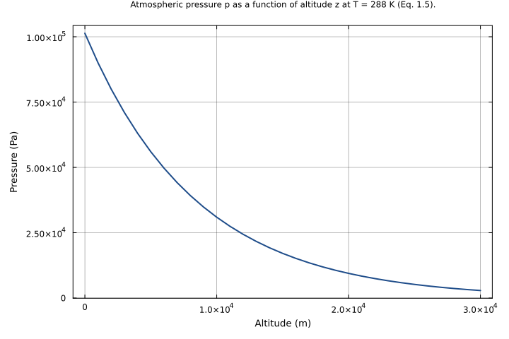
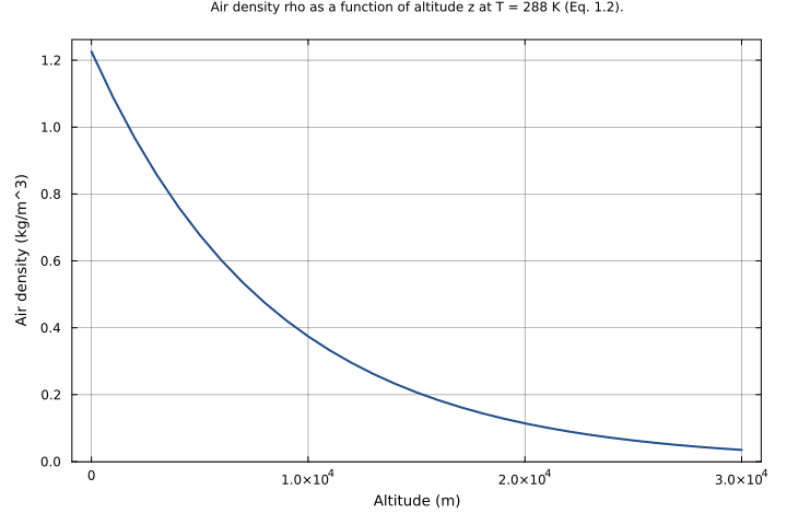
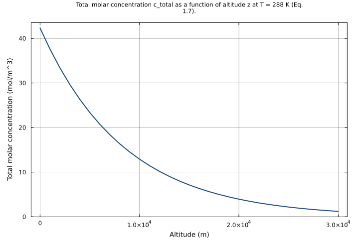
Upstream provides only structural (1.10 AtmosphericThermodynamics Composite Structure) and compilation (5.9 AtmosphericThermodynamics Compilation) tests for this component — no numerical-accuracy test. The inline tests here therefore anchor on physical reference values: standard sea-level conditions (z = 0, T = 288 K -> p = p_0, rho ~ 1.226 kg/m^3, c_total ~ 42.3 mol/m^3), the e-folding property at z = H (p = p_0/e), deep-decay altitudes, and cold/warm temperature columns. The H, p, rho values cross-check the sibling pressure_profile.esm (which shares the H / p / rho equations exactly): identical (z, T) cases give identical H, p, rho — sea_level_standard, one_scale_height, troposphere_10km, stratosphere_20km, cold_atmosphere_5km, warm_atmosphere_5km, and nonstandard_p0 all reuse pressure_profile.esm’s (z, T, p_0) inputs. The sea-level c_total ~ 42.3 mol/m^3 cross-checks total_molar_conc.esm (its std_sea_level case at T = 288.15 K gives 42.29 mol/m^3; the slightly lower T = 288 K used here gives the expected slightly higher 42.32 mol/m^3).
Tolerance rationale (model-level rel=1e-6): observed-only algebraic system (no ODE integration); 1e-6 covers float64 roundoff in the multiply/divide and exp(-z/H) expression chain across the altitude range (0-30 km) and the atmospheric temperature range (250-318 K)._
Parameters
| Name | Units | Default | Description |
|---|---|---|---|
z | m | 0.0 | Altitude above sea level (sea-level datum z = 0) |
T | K | 288.0 | Temperature of the isothermal atmospheric column — an input, assumed constant with altitude (sea-level standard 288 K) |
R | J/(mol*K) | 8.314 | Universal gas constant (Seinfeld & Pandis Appendix A) |
M_air | kg/mol | 0.02897 | Molecular weight of dry air (28.97 g/mol) |
g | m/s^2 | 9.807 | Gravitational acceleration |
p_0 | Pa | 101325.0 | Standard sea-level pressure (Seinfeld & Pandis Appendix A) |
Observed
| Name | Units | Default | Description |
|---|---|---|---|
H | m | Atmospheric scale height H = RT/(M_airg) — the altitude over which pressure falls by a factor e (Eq. 1.4) | |
p | Pa | Atmospheric pressure at altitude z (barometric formula, Eq. 1.5) | |
rho | kg/m^3 | Air density at altitude z (ideal gas law, Eq. 1.2) | |
c_total | mol/m^3 | Total molar concentration of air at altitude z (ideal gas law, Eq. 1.7) |
Observed expressions
$$ H = \frac{R \cdot T}{M_{air} \cdot g} $$Atmospheric scale height H = RT/(M_airg) — the altitude over which pressure falls by a factor e (Eq. 1.4)
$$ p = p_{0} \cdot e^{-\frac{z}{H}} $$Atmospheric pressure at altitude z (barometric formula, Eq. 1.5)
$$ rho = \frac{M_{air} \cdot p}{R \cdot T} $$Air density at altitude z (ideal gas law, Eq. 1.2)
$$ c_{total} = \frac{p}{R \cdot T} $$Total molar concentration of air at altitude z (ideal gas law, Eq. 1.7)
Analyses
thermodynamic_profile_vs_altitude
Pressure, density, and total molar concentration as a function of altitude for an isothermal atmosphere at the sea-level standard temperature (T = 288 K, H ~ 8428 m). Reproduces the canonical exponential decay of Seinfeld & Pandis Eqs. 1.5, 1.2, and 1.7 from the surface to 30 km.
Time span: 0.0 → 1.0
Swept over: z
c_total_over_altitude_and_temperature
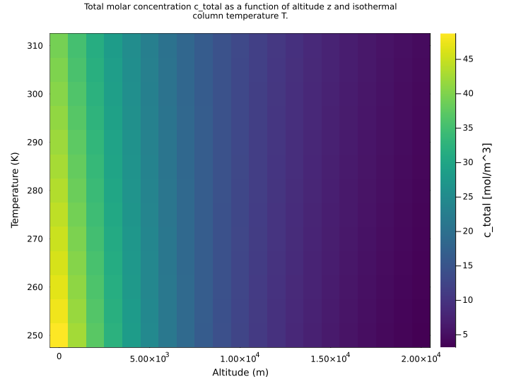
Two-dimensional sweep over altitude z (surface to 20 km) and the isothermal column temperature T (250-310 K). Surfaces the joint dependence of total molar concentration on altitude and on temperature: warmer columns have a larger scale height and so decay more slowly with altitude, while at fixed pressure colder air is denser in moles per volume.
Time span: 0.0 → 1.0
Swept over: z, T
Raw .esm
Raw .esm JSON (this component)
{
  "reference": {
    "notes": "source_ref: AtmosphericDynamics.jl@816cc391:src/seinfeld_pandis_ch1.jl:479\nUpstream `AtmosphericThermodynamics` is an MTK `@component` with R, M_air, g, p_0 as `@constants`, z as a `@parameter`, and T(t), H(t), p(t), rho(t), c_total(t) as `@variables`. It carries four algebraic equations (Seinfeld & Pandis Ch 1): H = R*T/(M_air*g) (Eq. 1.4), p = p_0*exp(-z/H) (Eq. 1.5), rho = M_air*p/(R*T) (Eq. 1.2), and c_total = p/(R*T) (Eq. 1.7), and returns `System(eqs, t; name)` with no subsystems.\n\nFlat model, not subsystem-composed: docs/migration-tracker.md line 346 lists this component with feature `coupling.couple` and `depends_on = IdealGasLaw, WaterVaporThermodynamics, AtmosphericPressureProfile`. Those annotations are derived from the upstream docstring (\"combines Equations 1.2, 1.4, 1.5, 1.7\"), not from the implementation: the `@component` does not instantiate any of those components as MTK subsystems — it re-derives the four equations inline. There is no `System(eqs, t; systems=[...])` call and no `couple` method anywhere in the source (the only subsystem composition in src/seinfeld_pandis_ch1.jl is the sibling `WaterVaporThermodynamics` at line 433, `System(eqs, t; systems=[sat, rh])`). It is therefore migrated as a flat algebraic model, mirroring the sibling pressure_profile.esm (AtmosphericPressureProfile, src/seinfeld_pandis_ch1.jl:151) — which has the identical structure and shares three of the same four equations — and NOT as a subsystem-composed model like water_vapor_thermo.esm.\n\nT appears only on equation right-hand sides — it is an input, not a computed output — so the four equations close exactly over the four states H, p, rho, c_total. For standalone serialization (and to make the component well-posed in isolation) T, z, R, M_air, g, and p_0 are declared as parameters here, leaving H, p, rho, c_total as the algebraic states. This matches the bead's `(L, observed-only)` classification in docs/migration-tracker.md and the IdealGasLaw / pressure_profile.esm / total_molar_conc.esm serialization pattern in this directory. The upstream `5.9 AtmosphericThermodynamics Compilation` test (test/seinfeld_pandis_ch1_test.jl:513) confirms this input/output split: it compiles the component with `inputs = [at_nns.T]`, leaving H, p, rho, c_total as the computed unknowns. Constant values (R = 8.314 J/(mol*K), M_air = 0.02897 kg/mol, g = 9.807 m/s^2, p_0 = 101325.0 Pa) come from the upstream module's R_GAS / M_AIR / G_ACCEL / P_0 (Seinfeld & Pandis Appendix A). The four algebraic equations are unchanged from upstream; `system_kind` is left unset (zero differential states), consistent with siblings pressure_profile.esm / total_molar_conc.esm / ideal_gas.esm.\n\nUpstream provides only structural (`1.10 AtmosphericThermodynamics Composite Structure`) and compilation (`5.9 AtmosphericThermodynamics Compilation`) tests for this component — no numerical-accuracy test. The inline `tests` here therefore anchor on physical reference values: standard sea-level conditions (z = 0, T = 288 K -> p = p_0, rho ~ 1.226 kg/m^3, c_total ~ 42.3 mol/m^3), the e-folding property at z = H (p = p_0/e), deep-decay altitudes, and cold/warm temperature columns. The H, p, rho values cross-check the sibling pressure_profile.esm (which shares the H / p / rho equations exactly): identical (z, T) cases give identical H, p, rho — sea_level_standard, one_scale_height, troposphere_10km, stratosphere_20km, cold_atmosphere_5km, warm_atmosphere_5km, and nonstandard_p0 all reuse pressure_profile.esm's (z, T, p_0) inputs. The sea-level c_total ~ 42.3 mol/m^3 cross-checks total_molar_conc.esm (its std_sea_level case at T = 288.15 K gives 42.29 mol/m^3; the slightly lower T = 288 K used here gives the expected slightly higher 42.32 mol/m^3).\n\nTolerance rationale (model-level rel=1e-6): observed-only algebraic system (no ODE integration); 1e-6 covers float64 roundoff in the multiply/divide and exp(-z/H) expression chain across the altitude range (0-30 km) and the atmospheric temperature range (250-318 K)."
  },
  "tolerance": {
    "rel": 1e-06
  },
  "variables": {
    "z": {
      "type": "parameter",
      "units": "m",
      "default": 0.0,
      "description": "Altitude above sea level (sea-level datum z = 0)"
    },
    "T": {
      "type": "parameter",
      "units": "K",
      "default": 288.0,
      "description": "Temperature of the isothermal atmospheric column — an input, assumed constant with altitude (sea-level standard 288 K)"
    },
    "R": {
      "type": "parameter",
      "units": "J/(mol*K)",
      "default": 8.314,
      "description": "Universal gas constant (Seinfeld & Pandis Appendix A)"
    },
    "M_air": {
      "type": "parameter",
      "units": "kg/mol",
      "default": 0.02897,
      "description": "Molecular weight of dry air (28.97 g/mol)"
    },
    "g": {
      "type": "parameter",
      "units": "m/s^2",
      "default": 9.807,
      "description": "Gravitational acceleration"
    },
    "p_0": {
      "type": "parameter",
      "units": "Pa",
      "default": 101325.0,
      "description": "Standard sea-level pressure (Seinfeld & Pandis Appendix A)"
    },
    "H": {
      "type": "unknown",
      "units": "m",
      "description": "Atmospheric scale height H = R*T/(M_air*g) — the altitude over which pressure falls by a factor e (Eq. 1.4)"
    },
    "p": {
      "type": "unknown",
      "units": "Pa",
      "description": "Atmospheric pressure at altitude z (barometric formula, Eq. 1.5)"
    },
    "rho": {
      "type": "unknown",
      "units": "kg/m^3",
      "description": "Air density at altitude z (ideal gas law, Eq. 1.2)"
    },
    "c_total": {
      "type": "unknown",
      "units": "mol/m^3",
      "description": "Total molar concentration of air at altitude z (ideal gas law, Eq. 1.7)"
    }
  },
  "equations": [
    {
      "_comment": "Eq. 1.4 - Atmospheric scale height: H = R*T/(M_air*g)",
      "lhs": "H",
      "rhs": {
        "op": "/",
        "args": [
          {
            "op": "*",
            "args": [
              "R",
              "T"
            ]
          },
          {
            "op": "*",
            "args": [
              "M_air",
              "g"
            ]
          }
        ]
      }
    },
    {
      "_comment": "Eq. 1.5 - Barometric formula (isothermal atmosphere): p = p_0*exp(-z/H)",
      "lhs": "p",
      "rhs": {
        "op": "*",
        "args": [
          "p_0",
          {
            "op": "exp",
            "args": [
              {
                "op": "-",
                "args": [
                  {
                    "op": "/",
                    "args": [
                      "z",
                      "H"
                    ]
                  }
                ]
              }
            ]
          }
        ]
      }
    },
    {
      "_comment": "Eq. 1.2 - Ideal gas law for air density: rho = M_air*p/(R*T)",
      "lhs": "rho",
      "rhs": {
        "op": "/",
        "args": [
          {
            "op": "*",
            "args": [
              "M_air",
              "p"
            ]
          },
          {
            "op": "*",
            "args": [
              "R",
              "T"
            ]
          }
        ]
      }
    },
    {
      "_comment": "Eq. 1.7 - Total molar concentration of air from the ideal gas law: c_total = p/(R*T)",
      "lhs": "c_total",
      "rhs": {
        "op": "/",
        "args": [
          "p",
          {
            "op": "*",
            "args": [
              "R",
              "T"
            ]
          }
        ]
      }
    }
  ],
  "tests": [
    {
      "id": "sea_level_standard",
      "description": "Standard sea-level reference (z = 0, T = 288 K). The barometric formula reduces to p = p_0 at the datum; the ideal gas law then gives the standard sea-level air density (~1.226 kg/m^3) and total molar concentration (~42.3 mol/m^3), and the scale height is H ~ 8428 m. This is the boundary condition the whole profile is anchored to. The system is algebraic, so c_total is also asserted at t = 1.0 to confirm time-invariance.",
      "parameter_overrides": {
        "z": 0.0,
        "T": 288.0
      },
      "time_span": {
        "start": 0.0,
        "end": 1.0
      },
      "assertions": [
        {
          "variable": "H",
          "time": 0.0,
          "expected": 8427.870183108378
        },
        {
          "variable": "p",
          "time": 0.0,
          "expected": 101325.0
        },
        {
          "variable": "rho",
          "time": 0.0,
          "expected": 1.2259213249739396
        },
        {
          "variable": "c_total",
          "time": 0.0,
          "expected": 42.31692526661856
        },
        {
          "variable": "c_total",
          "time": 1.0,
          "expected": 42.31692526661856
        }
      ]
    },
    {
      "id": "one_scale_height",
      "description": "At an altitude equal to the scale height (z = H(288 K) = 8427.87 m) the pressure falls by exactly a factor e: p = p_0/e ~ 37275 Pa. This is the defining property of the scale height (Seinfeld & Pandis Eq. 1.5); the expected H and p match pressure_profile.esm's one_scale_height case. The total molar concentration falls by the same factor e to ~15.6 mol/m^3.",
      "parameter_overrides": {
        "z": 8427.870183108378,
        "T": 288.0
      },
      "time_span": {
        "start": 0.0,
        "end": 1.0
      },
      "assertions": [
        {
          "variable": "H",
          "time": 0.0,
          "expected": 8427.870183108378
        },
        {
          "variable": "p",
          "time": 0.0,
          "expected": 37275.38437669639
        },
        {
          "variable": "c_total",
          "time": 0.0,
          "expected": 15.567526819177322
        }
      ]
    },
    {
      "id": "troposphere_10km",
      "description": "Upper-troposphere case at 10 km altitude (T = 288 K). With the isothermal scale height H ~ 8428 m the estimate is p ~ 309 mbar; the constant-H idealization overshoots the real ~265 mbar near this altitude (Seinfeld & Pandis Table 1.4). Exercises pressure, density, and total molar concentration well above the surface.",
      "parameter_overrides": {
        "z": 10000.0,
        "T": 288.0
      },
      "time_span": {
        "start": 0.0,
        "end": 1.0
      },
      "assertions": [
        {
          "variable": "p",
          "time": 0.0,
          "expected": 30932.07823850794
        },
        {
          "variable": "rho",
          "time": 0.0,
          "expected": 0.3742442076323634
        },
        {
          "variable": "c_total",
          "time": 0.0,
          "expected": 12.918336473329768
        }
      ]
    },
    {
      "id": "stratosphere_20km",
      "description": "Deep-decay case at 20 km altitude (z ~ 2.37 H, T = 288 K): pressure has fallen to ~9.4 kPa, density to ~0.114 kg/m^3, and total molar concentration to ~3.9 mol/m^3. Exercises the small-pressure tail of the exponential.",
      "parameter_overrides": {
        "z": 20000.0,
        "T": 288.0
      },
      "time_span": {
        "start": 0.0,
        "end": 1.0
      },
      "assertions": [
        {
          "variable": "p",
          "time": 0.0,
          "expected": 9442.817312145833
        },
        {
          "variable": "rho",
          "time": 0.0,
          "expected": 0.11424772870261707
        },
        {
          "variable": "c_total",
          "time": 0.0,
          "expected": 3.9436564964658984
        }
      ]
    },
    {
      "id": "cold_atmosphere_5km",
      "description": "Cold mid-troposphere column (T = 253 K) at z = 5 km. The lower temperature shrinks the scale height to H ~ 7404 m (cross-checked against pressure_profile.esm cold_atmosphere_5km), so pressure decays faster with altitude than the 288 K case and c_total is correspondingly higher at fixed pressure.",
      "parameter_overrides": {
        "z": 5000.0,
        "T": 253.0
      },
      "time_span": {
        "start": 0.0,
        "end": 1.0
      },
      "assertions": [
        {
          "variable": "H",
          "time": 0.0,
          "expected": 7403.649848355624
        },
        {
          "variable": "p",
          "time": 0.0,
          "expected": 51572.60347926007
        },
        {
          "variable": "c_total",
          "time": 0.0,
          "expected": 24.51819611820058
        }
      ]
    },
    {
      "id": "warm_atmosphere_5km",
      "description": "Warm column (T = 318 K, ~45 C) at z = 5 km. The higher temperature stretches the scale height to H ~ 9306 m (cross-checked against pressure_profile.esm warm_atmosphere_5km), so pressure decays more slowly with altitude than the 288 K case. With cold_atmosphere_5km this brackets the temperature dependence at fixed altitude.",
      "parameter_overrides": {
        "z": 5000.0,
        "T": 318.0
      },
      "time_span": {
        "start": 0.0,
        "end": 1.0
      },
      "assertions": [
        {
          "variable": "H",
          "time": 0.0,
          "expected": 9305.773327182167
        },
        {
          "variable": "p",
          "time": 0.0,
          "expected": 59206.55805835972
        },
        {
          "variable": "c_total",
          "time": 0.0,
          "expected": 22.394051580179116
        }
      ]
    },
    {
      "id": "nonstandard_p0",
      "description": "Non-default sea-level pressure (p_0 = 100000 Pa) at z = 5 km, T = 288 K. Verifies p scales linearly with p_0 while the exponential decay factor stays fixed; density rho = M_air*p/(R*T) and total molar concentration c_total = p/(R*T) both follow p proportionally.",
      "parameter_overrides": {
        "z": 5000.0,
        "T": 288.0,
        "p_0": 100000.0
      },
      "time_span": {
        "start": 0.0,
        "end": 1.0
      },
      "assertions": [
        {
          "variable": "p",
          "time": 0.0,
          "expected": 55251.776171869395
        },
        {
          "variable": "rho",
          "time": 0.0,
          "expected": 0.6684858687567893
        },
        {
          "variable": "c_total",
          "time": 0.0,
          "expected": 23.075107654704496
        }
      ]
    }
  ],
  "analyses": [
    {
      "id": "thermodynamic_profile_vs_altitude",
      "description": "Pressure, density, and total molar concentration as a function of altitude for an isothermal atmosphere at the sea-level standard temperature (T = 288 K, H ~ 8428 m). Reproduces the canonical exponential decay of Seinfeld & Pandis Eqs. 1.5, 1.2, and 1.7 from the surface to 30 km.",
      "initial_state": {},
      "parameters": {
        "T": 288.0
      },
      "time_span": {
        "start": 0.0,
        "end": 1.0
      },
      "parameter_sweep": {
        "type": "cartesian",
        "dimensions": [
          {
            "parameter": "z",
            "range": {
              "start": 0.0,
              "stop": 30000.0,
              "count": 31,
              "scale": "linear"
            }
          }
        ]
      },
      "plots": [
        {
          "id": "p_vs_z",
          "type": "line",
          "description": "Atmospheric pressure p as a function of altitude z at T = 288 K (Eq. 1.5).",
          "x": {
            "variable": "z",
            "label": "Altitude (m)"
          },
          "y": {
            "variable": "p",
            "label": "Pressure (Pa)"
          }
        },
        {
          "id": "rho_vs_z",
          "type": "line",
          "description": "Air density rho as a function of altitude z at T = 288 K (Eq. 1.2).",
          "x": {
            "variable": "z",
            "label": "Altitude (m)"
          },
          "y": {
            "variable": "rho",
            "label": "Air density (kg/m^3)"
          }
        },
        {
          "id": "c_total_vs_z",
          "type": "line",
          "description": "Total molar concentration c_total as a function of altitude z at T = 288 K (Eq. 1.7).",
          "x": {
            "variable": "z",
            "label": "Altitude (m)"
          },
          "y": {
            "variable": "c_total",
            "label": "Total molar concentration (mol/m^3)"
          }
        }
      ]
    },
    {
      "id": "c_total_over_altitude_and_temperature",
      "description": "Two-dimensional sweep over altitude z (surface to 20 km) and the isothermal column temperature T (250-310 K). Surfaces the joint dependence of total molar concentration on altitude and on temperature: warmer columns have a larger scale height and so decay more slowly with altitude, while at fixed pressure colder air is denser in moles per volume.",
      "initial_state": {},
      "parameters": {},
      "time_span": {
        "start": 0.0,
        "end": 1.0
      },
      "parameter_sweep": {
        "type": "cartesian",
        "dimensions": [
          {
            "parameter": "z",
            "range": {
              "start": 0.0,
              "stop": 20000.0,
              "count": 21,
              "scale": "linear"
            }
          },
          {
            "parameter": "T",
            "range": {
              "start": 250.0,
              "stop": 310.0,
              "count": 13,
              "scale": "linear"
            }
          }
        ]
      },
      "plots": [
        {
          "id": "c_total_heatmap",
          "type": "heatmap",
          "description": "Total molar concentration c_total as a function of altitude z and isothermal column temperature T.",
          "x": {
            "variable": "z",
            "label": "Altitude (m)"
          },
          "y": {
            "variable": "T",
            "label": "Temperature (K)"
          },
          "value": {
            "variable": "c_total",
            "reduce": "final"
          }
        }
      ]
    }
  ]
}