LocalScaleMeteorology
Local-scale boundary-layer meteorology from Seinfeld & Pandis (2006) "Atmospheric Chemistry and Physics", 2nd ed., Chapter 16 "Meteorology of the Local Scale". A flat observed-only algebraic component that combines atmospheric static-stability analysis, Monin-Obukhov surface-layer similarity theory and Pasquill stability-class estimation: from the air temperature and pressure, the surface-layer geometry, the friction velocity u_star and the surface sensible heat flux q_z it computes the potential temperature θ (Eq. 16.14), the actual and potential-temperature lapse rates dT_dz and dθ_dz (Eqs. 16.16-16.18), the Monin-Obukhov length L and its inverse L_inv (Eq. 16.70), the stability parameter ζ = z/L, the Businger-Dyer stability functions φ_m, φ_h and their integrated forms ψ_m, ψ_h (Eqs. 16.75, 16.78-16.79), the stability-corrected mean wind speed ū (Eq. 16.66) and the Pasquill stability class (1=A to 6=F) via the Golder (1972) correlation (Eq. 16.83). Twelve purely-algebraic equations, no time integration. Migrated from AtmosphericDynamics.jl@816cc391 src/local_scale_meteorology.jl:234 (`LocalScaleMeteorology` @component).
Description
Local-scale boundary-layer meteorology from Seinfeld & Pandis (2006) “Atmospheric Chemistry and Physics”, 2nd ed., Chapter 16 “Meteorology of the Local Scale”. A flat observed-only algebraic component that combines atmospheric static-stability analysis, Monin-Obukhov surface-layer similarity theory and Pasquill stability-class estimation: from the air temperature and pressure, the surface-layer geometry, the friction velocity u_star and the surface sensible heat flux q_z it computes the potential temperature θ (Eq. 16.14), the actual and potential-temperature lapse rates dT_dz and dθ_dz (Eqs. 16.16-16.18), the Monin-Obukhov length L and its inverse L_inv (Eq. 16.70), the stability parameter ζ = z/L, the Businger-Dyer stability functions φ_m, φ_h and their integrated forms ψ_m, ψ_h (Eqs. 16.75, 16.78-16.79), the stability-corrected mean wind speed ū (Eq. 16.66) and the Pasquill stability class (1=A to 6=F) via the Golder (1972) correlation (Eq. 16.83). Twelve purely-algebraic equations, no time integration. Migrated from AtmosphericDynamics.jl@816cc391 src/local_scale_meteorology.jl:234 (LocalScaleMeteorology @component).
Reference
_source_ref: AtmosphericDynamics.jl@816cc3918e1eef2c2ee6d8fa8dd73c8f13a85a47:src/local_scale_meteorology.jl:234
Upstream LocalScaleMeteorology is a ModelingToolkit @component that combines the atmospheric static-stability diagnostics of the sibling AtmosphericStability component and the Monin-Obukhov surface-layer similarity theory of SurfaceLayerProfile with a Pasquill stability-class estimate, all from Seinfeld & Pandis (2006) Ch. 16 (Meteorology of the Local Scale, pp. 720-760). It declares 18 referenced @constants, 10 @parameters, 12 @variables and 12 equations, returning System(eqs, t; name).
Flat single model – NOT a coupling.couple composition. docs/migration-tracker.md tags this row features: variables, parameters, coupling.couple with depends_on: AtmosphericStability, SurfaceLayerProfile, and the upstream docstring calls it a “composite system”. The upstream code, however, builds a plain System(eqs, t; name) with all 12 equations written inline (src/local_scale_meteorology.jl:308-374): it does NOT call System(...; systems=[...]) and constructs no subcomponents – it re-implements the AtmosphericStability and SurfaceLayerProfile physics directly. The migration therefore represents it as a single flat model with a 12-equation block, not as an ESS subsystem-composed model; the tracker depends_on entries record conceptual provenance (the sibling components whose physics is reused), not a structural dependency. The shared equations are byte-identical to the corresponding equations of the gate-verified sibling migrations stability.esm and surface_layer_profile.esm.
System kind: all 12 equations are explicit algebraic assignments (lhs ~ rhs) with no D(.) operator – every output is a closed-form expression of the inputs. system_kind is left unset (default ‘ode’); the compiled system has zero differential states, exactly as for the siblings stability.esm and surface_layer_profile.esm.
Variable classification. (1) T, T_below, p, z, z₀, Δz, T₀, ρ, u_star, q_z: upstream MTK @parameters – the external inputs – encoded type: parameter with their upstream defaults. (2) θ, dT_dz, dθ_dz, L, ζ, φ_m, φ_h, ψ_m, ψ_h, ū, L_inv, pasquill_class: upstream @variables, each the LHS of exactly one purely-algebraic equation – observed algebraic outputs with no time derivative and hence no initial condition – encoded type: state with no default. (3) g, κ, ĉ_p, R_air, p₀, Γ_d, ε_q, z₀_ref and the 10 Golder coefficients: upstream MTK @constants; the ESS schema has no constant variable type, so each is encoded type: parameter carrying its upstream value as default, exactly as in stability.esm and surface_layer_profile.esm.
Omitted constants a_D, b_D. Upstream declares 12 Golder (1972) coefficient @constants a_A, b_A, …, a_F, b_F (src lines 251-262). The pasquill_class equation (src lines 358-373) is a 5-level nested ifelse; its fourth branch – the class-D / neutral boundary – is compared against the class-E coefficients a_E + b_E*log10(z₀/z₀_ref) (src line 365), so a_D and b_D (both declared 0.0) appear in no equation. An unreferenced MTK @constant is not collected into the built System (the same reason g is omitted from stability.esm), so a_D and b_D are omitted here; the remaining 10 Golder coefficients are all referenced and retained. The upstream LocalScaleMeteorology structure testitem checks only length(equations(sys)) == 12 and a handful of named parameters, consistent with this.
κ_exp local. Upstream binds a plain Julia local κ_exp = R_air / ĉ_p (~ 0.286, the Poisson exponent R/c_p) and uses it as the exponent of the potential-temperature equation (Eq. 16.14). MTK inlines it when System(eqs, t) is built; the .esm mirrors this, writing equation 1’s exponent as the sub-expression R_air / ĉ_p.
Equation faithfulness. The 12 upstream equations (src lines 308-374) are preserved in upstream order: θ (Eq. 16.14), dT_dz (finite-difference actual lapse rate), dθ_dz (Eqs. 16.16-16.18), L (Eq. 16.70), L_inv = 1/L, ζ = z/L, φ_m and φ_h (Eq. 16.75 Businger-Dyer), ψ_m and ψ_h (Eqs. 16.78-16.79), ū (Eq. 16.66 with the Eq. 16.77 correction), and pasquill_class (Eq. 16.83 Golder correlation). The L, ζ, φ_m, φ_h, ψ_m, ψ_h and ū equation trees are copied verbatim from the sibling surface_layer_profile.esm, where mtk2esm reordered the commutative */+ operands of L, rewrote x^(-n) as 1/x^n in φ_m/φ_h, folded ((1-15ζ)^0.25)^2 to (1-15ζ)^0.5 in ψ_m/ψ_h, and folded the π/2 term of ψ_m to the float literal 1.5707963267948966. The θ, dT_dz and dθ_dz trees match the corresponding stability.esm equations.
Identifiers. Upstream Unicode identifiers are kept verbatim (θ, dθ_dz, Γ_d, p₀, Δz, ĉ_p, κ, ε_q, z₀, z₀_ref, T₀, ρ, ζ, φ_m, φ_h, ψ_m, ψ_h, ū), matching surface_layer_profile.esm. R_air is the dry-air specific gas constant in J/(kgK); it is named R_air rather than the schema-reserved bare name R, correct since it is dimensionally J/(kgK), not the universal gas constant in J/(mol*K).
Units are SI-coherent and carried verbatim from the upstream declarations; they are descriptive metadata (the ESS runners perform no dimensional analysis).
Tolerance rationale (model-level rel=1.0e-6). The system is a closed-form algebraic evaluation – no ODE integration, no implicit solve – so there is no integrator error to bound; rel=1.0e-6 covers float64 round-off and cross-runner libm differences in the ^/log/log10/atan chain, matching the siblings. Near-zero outputs in the neutral regime – ζ, L_inv, ψ_m, ψ_h ~ 1e-12..1e-14 at the default q_z = 0, where the ε_q heat-flux regularization makes |L| enormous – carry a per-assertion abs=1.0e-6; the exact-zero actual lapse rate dT_dz (T = T_below) carries abs=1.0e-12.
Test reproduction. The 10 inline tests reproduce every LocalScaleMeteorology scenario of test/local_scale_meteorology_test.jl plus the AtmosphericDynamics.jl docs “Complete Boundary Layer Analysis” example: defaults_baseline exercises all 12 outputs at the declared defaults (the upstream LocalScaleMeteorology structure testitem); potential_temp_850hPa and potential_temp_cold_low_pressure reproduce the Potential temperature and Physical constraints θ checks; pasquill_unstable_class_C and pasquill_stable_class_F reproduce the two Pasquill stability classification testitems (the upstream <= 3 / >= 4 assertions become the exact classes 3 and 6); physical_constraints_wind_class_D reproduces the Physical constraints ū > 0 check. The added scenarios light_wind_strong_heating_class_A, moderately_unstable_class_B and inversion_stable_class_E extend Pasquill coverage to classes 1, 2 and 5 (the suite spans the full A-F range) and exercise the inversion (dT_dz > 0) and stable-branch (ζ > 0) cases; summer_afternoon_boundary_layer reproduces the docs composite example. Expected values are the float64 results of the upstream formulas; the L/ζ/φ/ψ/ū values of the default and summer-afternoon scenarios agree with the corresponding surface_layer_profile.esm tests, as those equations are shared verbatim.
Examples. The 3 examples reproduce AtmosphericDynamics.jl docs figures (docs/src/local_scale_meteorology.md): potential_temperature_profile sweeps pressure p (the Potential Temperature Profile figure); monin_obukhov_length_vs_heat_flux sweeps the surface heat flux q_z over the unstable regime (the Monin-Obukhov Length vs Heat Flux figure); pasquill_class_vs_roughness_length sweeps the roughness length z₀ at a fixed unstable heat flux to trace the discrete Pasquill A-F classification against the Golder (1972) z₀ correlation (the Monin-Obukhov Length vs Roughness Length for Pasquill Stability Classes figure), the diagnostic distinctive to this composite component. All three example sweeps stay in the unstable / neutral regime (ζ <= 0); the example renderer eagerly evaluates both ifelse branches, and the Businger-Dyer unstable branch (1-15ζ)^(-1/4) is real-valued only for ζ <= 0._
Parameters
| Name | Units | Default | Description |
|---|---|---|---|
T | K | 288.15 | Air temperature at height z |
T_below | K | 288.15 | Air temperature at height z - Δz |
p | Pa | 101325.0 | Pressure at height z |
z | m | 10.0 | Height above ground |
z₀ | m | 0.1 | Roughness length (Table 16.1) |
Δz | m | 100.0 | Vertical spacing for gradient calculation |
T₀ | K | 288.15 | Reference temperature (surface) |
ρ | kg/m^3 | 1.225 | Air density |
u_star | m/s | 0.3 | Friction velocity |
q_z | W/m^2 | 0.0 | Surface sensible heat flux (positive upward) |
g | m/s^2 | 9.807 | Gravitational acceleration |
κ | 1 | 0.4 | von Karman constant (dimensionless) |
ĉ_p | J/(kg*K) | 1005.0 | Specific heat of air at constant pressure |
R_air | J/(kg*K) | 287.0 | Gas constant for dry air |
p₀ | Pa | 101325.0 | Reference pressure (sea level) |
Γ_d | K/m | 0.00976 | Dry adiabatic lapse rate (Eq. 16.8: g/c_p = 9.807/1005 ≈ 9.76 K/km) |
ε_q | W/m^2 | 1e-10 | Small regularization for heat flux |
z₀_ref | m | 1.0 | Reference length for dimensionless log |
a_A | m^-1 | -0.096 | Golder (1972) coefficient a for Pasquill class A (Eq. 16.83: 1/L = a + b·log₁₀(z₀)) |
b_A | m^-1 | 0.029 | Golder (1972) coefficient b for Pasquill class A (Eq. 16.83: 1/L = a + b·log₁₀(z₀)) |
a_B | m^-1 | -0.037 | Golder (1972) coefficient a for Pasquill class B (Eq. 16.83: 1/L = a + b·log₁₀(z₀)) |
b_B | m^-1 | 0.029 | Golder (1972) coefficient b for Pasquill class B (Eq. 16.83: 1/L = a + b·log₁₀(z₀)) |
a_C | m^-1 | -0.002 | Golder (1972) coefficient a for Pasquill class C (Eq. 16.83: 1/L = a + b·log₁₀(z₀)) |
b_C | m^-1 | 0.018 | Golder (1972) coefficient b for Pasquill class C (Eq. 16.83: 1/L = a + b·log₁₀(z₀)) |
a_E | m^-1 | 0.004 | Golder (1972) coefficient a for Pasquill class E (Eq. 16.83: 1/L = a + b·log₁₀(z₀)) |
b_E | m^-1 | -0.018 | Golder (1972) coefficient b for Pasquill class E (Eq. 16.83: 1/L = a + b·log₁₀(z₀)) |
a_F | m^-1 | 0.035 | Golder (1972) coefficient a for Pasquill class F (Eq. 16.83: 1/L = a + b·log₁₀(z₀)) |
b_F | m^-1 | -0.036 | Golder (1972) coefficient b for Pasquill class F (Eq. 16.83: 1/L = a + b·log₁₀(z₀)) |
Observed
| Name | Units | Default | Description |
|---|---|---|---|
θ | K | Potential temperature (Eq. 16.14) | |
dT_dz | K/m | Actual temperature lapse rate | |
dθ_dz | K/m | Potential temperature gradient | |
L | m | Monin-Obukhov length (Eq. 16.70) | |
ζ | 1 | Stability parameter z/L (dimensionless) | |
φ_m | 1 | Momentum stability function (Eq. 16.75) (dimensionless) | |
φ_h | 1 | Heat stability function (Eq. 16.75) (dimensionless) | |
ψ_m | 1 | Integrated momentum stability function (dimensionless) | |
ψ_h | 1 | Integrated heat stability function (dimensionless) | |
ū | m/s | Mean wind speed at height z (Eq. 16.66) | |
L_inv | m^-1 | Inverse Monin-Obukhov length | |
pasquill_class | 1 | Pasquill stability class (1=A to 6=F) (dimensionless) |
Observed expressions
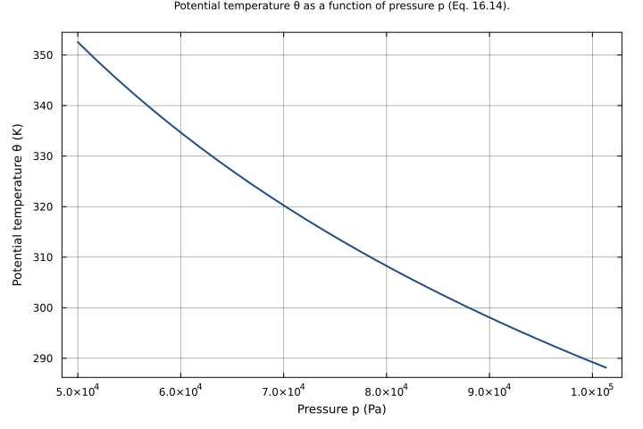
$$ θ = T \cdot \frac{p₀}{p}^{\frac{R_{air}}{ĉ_{p}}} $$Potential temperature (Eq. 16.14)
$$ dT_{dz} = \frac{T - T_{below}}{Δz} $$Actual temperature lapse rate
$$ dθ_{dz} = dT_{dz} + Γ_{d} $$Potential temperature gradient
$$ L = \frac{\left(-1\right) \cdot ĉ_{p} \cdot ρ \cdot u_{star}^{3} \cdot T₀}{κ \cdot g \cdot \left(q_{z} + ε_{q}\right)} $$Monin-Obukhov length (Eq. 16.70)
$$ ζ = \frac{z}{L} $$Stability parameter z/L (dimensionless)
$$ φ_{m} = \mathrm{ifelse}\left(\mathrm{<}\left(ζ, 0\right), \frac{1}{\left(1 + \left(-15\right) \cdot ζ\right)^{0.25}}, 1 + 4.7 \cdot ζ\right) $$Momentum stability function (Eq. 16.75) (dimensionless)
$$ φ_{h} = \mathrm{ifelse}\left(\mathrm{<}\left(ζ, 0\right), \frac{1}{\left(1 + \left(-15\right) \cdot ζ\right)^{0.5}}, 1 + 4.7 \cdot ζ\right) $$Heat stability function (Eq. 16.75) (dimensionless)
$$ ψ_{m} = \mathrm{ifelse}\left(\mathrm{<}\left(ζ, 0\right), 1.5707963267948966 + \left(-2\right) \cdot \mathrm{atan}\left(\left(1 + \left(-15\right) \cdot ζ\right)^{0.25}\right) + 2 \cdot \ln\left(\frac{1 + \left(1 + \left(-15\right) \cdot ζ\right)^{0.25}}{2}\right) + \ln\left(\frac{1 + \left(1 + \left(-15\right) \cdot ζ\right)^{0.5}}{2}\right), \left(-4.7\right) \cdot ζ\right) $$Integrated momentum stability function (dimensionless)
$$ ψ_{h} = \mathrm{ifelse}\left(\mathrm{<}\left(ζ, 0\right), 2 \cdot \ln\left(\frac{1 + \left(1 + \left(-15\right) \cdot ζ\right)^{0.5}}{2}\right), \left(-4.7\right) \cdot ζ\right) $$Integrated heat stability function (dimensionless)
$$ ū = \frac{\left(\left(-1\right) \cdot ψ_{m} + \ln\left(\frac{z}{z₀}\right)\right) \cdot u_{star}}{κ} $$Mean wind speed at height z (Eq. 16.66)
$$ L_{inv} = \frac{1}{L} $$Inverse Monin-Obukhov length
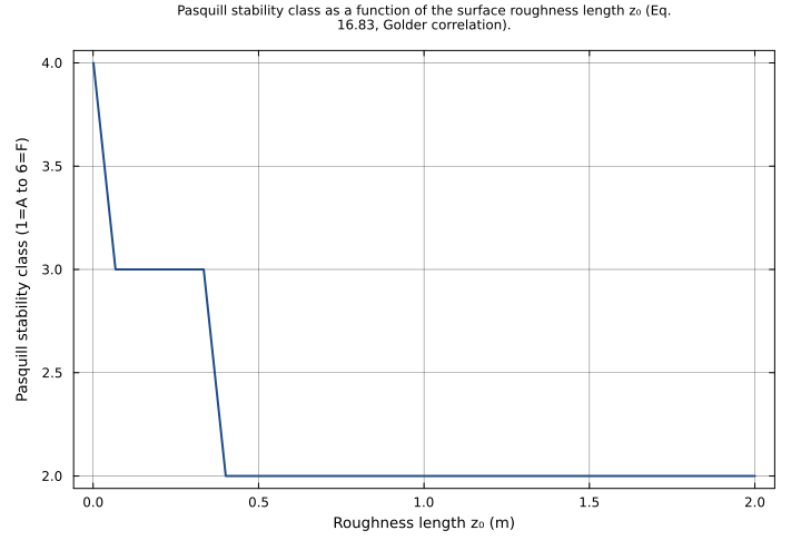
$$ pasquill_{class} = \mathrm{ifelse}\left(\mathrm{<}\left(L_{inv}, a_{A} + b_{A} \cdot \log_{10}\left(\frac{z₀}{z₀_{ref}}\right)\right), 1, \mathrm{ifelse}\left(\mathrm{<}\left(L_{inv}, a_{B} + b_{B} \cdot \log_{10}\left(\frac{z₀}{z₀_{ref}}\right)\right), 2, \mathrm{ifelse}\left(\mathrm{<}\left(L_{inv}, a_{C} + b_{C} \cdot \log_{10}\left(\frac{z₀}{z₀_{ref}}\right)\right), 3, \mathrm{ifelse}\left(\mathrm{<}\left(L_{inv}, a_{E} + b_{E} \cdot \log_{10}\left(\frac{z₀}{z₀_{ref}}\right)\right), 4, \mathrm{ifelse}\left(\mathrm{<}\left(L_{inv}, a_{F} + b_{F} \cdot \log_{10}\left(\frac{z₀}{z₀_{ref}}\right)\right), 5, 6\right)\right)\right)\right)\right) $$Pasquill stability class (1=A to 6=F) (dimensionless)
Analyses
potential_temperature_profile
Potential temperature θ = T·(p₀/p)^(R_air/ĉ_p) (Eq. 16.14) swept over pressure p from 50000 to 101325 Pa at the default temperature T = 288.15 K. Reproduces the AtmosphericDynamics.jl docs Potential Temperature Profile figure — at fixed temperature θ rises as pressure falls, equalling the actual temperature at the sea-level reference pressure p₀ and exceeding it aloft where the (p₀/p) adiabatic-compression factor is greater than one.
Time span: 0.0 → 1.0
Swept over: p
monin_obukhov_length_vs_heat_flux
Monin-Obukhov length L (Eq. 16.70) as a function of the surface sensible heat flux q_z over the unstable regime (q_z > 0, surface heating), at the default u_star = 0.3 m/s. Reproduces the unstable branch of the AtmosphericDynamics.jl docs Monin-Obukhov Length vs Heat Flux figure: L is negative and grows toward 0 as the heat flux increases.
Time span: 0.0 → 1.0
Swept over: q_z

pasquill_class_vs_roughness_length
Pasquill stability class (1=A to 6=F) as a function of the surface roughness length z₀, swept from 0.001 to 2 m (Table 16.1, snow through low-density residential terrain) at a fixed moderately unstable surface heat flux q_z = 120 W/m^2 and the default u_star = 0.3 m/s. The Monin-Obukhov length L (and hence L_inv) is independent of z₀, so this example isolates the z₀ dependence of the Golder (1972) correlation (Eq. 16.83, 1/L = a + b·log₁₀(z₀)): as the surface roughens the class boundaries shift and the diagnosed Pasquill class steps between the unstable categories. Reproduces the AtmosphericDynamics.jl docs Monin-Obukhov Length vs Roughness Length for Pasquill Stability Classes figure.
Time span: 0.0 → 1.0
Swept over: z₀
Raw .esm
Raw .esm JSON (this component)
{
"reference": {
"notes": "source_ref: AtmosphericDynamics.jl@816cc3918e1eef2c2ee6d8fa8dd73c8f13a85a47:src/local_scale_meteorology.jl:234\n\nUpstream `LocalScaleMeteorology` is a ModelingToolkit `@component` that combines the atmospheric static-stability diagnostics of the sibling `AtmosphericStability` component and the Monin-Obukhov surface-layer similarity theory of `SurfaceLayerProfile` with a Pasquill stability-class estimate, all from Seinfeld & Pandis (2006) Ch. 16 (Meteorology of the Local Scale, pp. 720-760). It declares 18 referenced `@constants`, 10 `@parameters`, 12 `@variables` and 12 equations, returning `System(eqs, t; name)`.\n\nFlat single model -- NOT a coupling.couple composition. docs/migration-tracker.md tags this row `features: variables, parameters, coupling.couple` with `depends_on: AtmosphericStability, SurfaceLayerProfile`, and the upstream docstring calls it a \"composite system\". The upstream code, however, builds a plain `System(eqs, t; name)` with all 12 equations written inline (src/local_scale_meteorology.jl:308-374): it does NOT call `System(...; systems=[...])` and constructs no subcomponents -- it re-implements the AtmosphericStability and SurfaceLayerProfile physics directly. The migration therefore represents it as a single flat model with a 12-equation block, not as an ESS subsystem-composed model; the tracker `depends_on` entries record conceptual provenance (the sibling components whose physics is reused), not a structural dependency. The shared equations are byte-identical to the corresponding equations of the gate-verified sibling migrations stability.esm and surface_layer_profile.esm.\n\nSystem kind: all 12 equations are explicit algebraic assignments (lhs ~ rhs) with no `D(.)` operator -- every output is a closed-form expression of the inputs. `system_kind` is left unset (default 'ode'); the compiled system has zero differential states, exactly as for the siblings stability.esm and surface_layer_profile.esm.\n\nVariable classification. (1) T, T_below, p, z, z₀, Δz, T₀, ρ, u_star, q_z: upstream MTK `@parameters` -- the external inputs -- encoded type: parameter with their upstream defaults. (2) θ, dT_dz, dθ_dz, L, ζ, φ_m, φ_h, ψ_m, ψ_h, ū, L_inv, pasquill_class: upstream `@variables`, each the LHS of exactly one purely-algebraic equation -- observed algebraic outputs with no time derivative and hence no initial condition -- encoded type: state with no default. (3) g, κ, ĉ_p, R_air, p₀, Γ_d, ε_q, z₀_ref and the 10 Golder coefficients: upstream MTK `@constants`; the ESS schema has no `constant` variable type, so each is encoded type: parameter carrying its upstream value as default, exactly as in stability.esm and surface_layer_profile.esm.\n\nOmitted constants a_D, b_D. Upstream declares 12 Golder (1972) coefficient `@constants` a_A, b_A, ..., a_F, b_F (src lines 251-262). The pasquill_class equation (src lines 358-373) is a 5-level nested `ifelse`; its fourth branch -- the class-D / neutral boundary -- is compared against the class-E coefficients a_E + b_E*log10(z₀/z₀_ref) (src line 365), so a_D and b_D (both declared 0.0) appear in no equation. An unreferenced MTK `@constant` is not collected into the built `System` (the same reason g is omitted from stability.esm), so a_D and b_D are omitted here; the remaining 10 Golder coefficients are all referenced and retained. The upstream `LocalScaleMeteorology structure` testitem checks only `length(equations(sys)) == 12` and a handful of named parameters, consistent with this.\n\nκ_exp local. Upstream binds a plain Julia local `κ_exp = R_air / ĉ_p` (~ 0.286, the Poisson exponent R/c_p) and uses it as the exponent of the potential-temperature equation (Eq. 16.14). MTK inlines it when `System(eqs, t)` is built; the .esm mirrors this, writing equation 1's exponent as the sub-expression R_air / ĉ_p.\n\nEquation faithfulness. The 12 upstream equations (src lines 308-374) are preserved in upstream order: θ (Eq. 16.14), dT_dz (finite-difference actual lapse rate), dθ_dz (Eqs. 16.16-16.18), L (Eq. 16.70), L_inv = 1/L, ζ = z/L, φ_m and φ_h (Eq. 16.75 Businger-Dyer), ψ_m and ψ_h (Eqs. 16.78-16.79), ū (Eq. 16.66 with the Eq. 16.77 correction), and pasquill_class (Eq. 16.83 Golder correlation). The L, ζ, φ_m, φ_h, ψ_m, ψ_h and ū equation trees are copied verbatim from the sibling surface_layer_profile.esm, where `mtk2esm` reordered the commutative */+ operands of L, rewrote x^(-n) as 1/x^n in φ_m/φ_h, folded ((1-15ζ)^0.25)^2 to (1-15ζ)^0.5 in ψ_m/ψ_h, and folded the π/2 term of ψ_m to the float literal 1.5707963267948966. The θ, dT_dz and dθ_dz trees match the corresponding stability.esm equations.\n\nIdentifiers. Upstream Unicode identifiers are kept verbatim (θ, dθ_dz, Γ_d, p₀, Δz, ĉ_p, κ, ε_q, z₀, z₀_ref, T₀, ρ, ζ, φ_m, φ_h, ψ_m, ψ_h, ū), matching surface_layer_profile.esm. R_air is the dry-air specific gas constant in J/(kg*K); it is named R_air rather than the schema-reserved bare name R, correct since it is dimensionally J/(kg*K), not the universal gas constant in J/(mol*K).\n\nUnits are SI-coherent and carried verbatim from the upstream declarations; they are descriptive metadata (the ESS runners perform no dimensional analysis).\n\nTolerance rationale (model-level rel=1.0e-6). The system is a closed-form algebraic evaluation -- no ODE integration, no implicit solve -- so there is no integrator error to bound; rel=1.0e-6 covers float64 round-off and cross-runner libm differences in the ^/log/log10/atan chain, matching the siblings. Near-zero outputs in the neutral regime -- ζ, L_inv, ψ_m, ψ_h ~ 1e-12..1e-14 at the default q_z = 0, where the ε_q heat-flux regularization makes |L| enormous -- carry a per-assertion abs=1.0e-6; the exact-zero actual lapse rate dT_dz (T = T_below) carries abs=1.0e-12.\n\nTest reproduction. The 10 inline tests reproduce every LocalScaleMeteorology scenario of test/local_scale_meteorology_test.jl plus the AtmosphericDynamics.jl docs \"Complete Boundary Layer Analysis\" example: `defaults_baseline` exercises all 12 outputs at the declared defaults (the upstream `LocalScaleMeteorology structure` testitem); `potential_temp_850hPa` and `potential_temp_cold_low_pressure` reproduce the `Potential temperature` and `Physical constraints` θ checks; `pasquill_unstable_class_C` and `pasquill_stable_class_F` reproduce the two `Pasquill stability classification` testitems (the upstream <= 3 / >= 4 assertions become the exact classes 3 and 6); `physical_constraints_wind_class_D` reproduces the `Physical constraints` ū > 0 check. The added scenarios `light_wind_strong_heating_class_A`, `moderately_unstable_class_B` and `inversion_stable_class_E` extend Pasquill coverage to classes 1, 2 and 5 (the suite spans the full A-F range) and exercise the inversion (dT_dz > 0) and stable-branch (ζ > 0) cases; `summer_afternoon_boundary_layer` reproduces the docs composite example. Expected values are the float64 results of the upstream formulas; the L/ζ/φ/ψ/ū values of the default and summer-afternoon scenarios agree with the corresponding surface_layer_profile.esm tests, as those equations are shared verbatim.\n\nExamples. The 3 examples reproduce AtmosphericDynamics.jl docs figures (docs/src/local_scale_meteorology.md): `potential_temperature_profile` sweeps pressure p (the `Potential Temperature Profile` figure); `monin_obukhov_length_vs_heat_flux` sweeps the surface heat flux q_z over the unstable regime (the `Monin-Obukhov Length vs Heat Flux` figure); `pasquill_class_vs_roughness_length` sweeps the roughness length z₀ at a fixed unstable heat flux to trace the discrete Pasquill A-F classification against the Golder (1972) z₀ correlation (the `Monin-Obukhov Length vs Roughness Length for Pasquill Stability Classes` figure), the diagnostic distinctive to this composite component. All three example sweeps stay in the unstable / neutral regime (ζ <= 0); the example renderer eagerly evaluates both `ifelse` branches, and the Businger-Dyer unstable branch (1-15ζ)^(-1/4) is real-valued only for ζ <= 0."
},
"tolerance": {
"rel": 1e-06
},
"variables": {
"T": {
"type": "parameter",
"units": "K",
"default": 288.15,
"description": "Air temperature at height z"
},
"T_below": {
"type": "parameter",
"units": "K",
"default": 288.15,
"description": "Air temperature at height z - Δz"
},
"p": {
"type": "parameter",
"units": "Pa",
"default": 101325.0,
"description": "Pressure at height z"
},
"z": {
"type": "parameter",
"units": "m",
"default": 10.0,
"description": "Height above ground"
},
"z₀": {
"type": "parameter",
"units": "m",
"default": 0.1,
"description": "Roughness length (Table 16.1)"
},
"Δz": {
"type": "parameter",
"units": "m",
"default": 100.0,
"description": "Vertical spacing for gradient calculation"
},
"T₀": {
"type": "parameter",
"units": "K",
"default": 288.15,
"description": "Reference temperature (surface)"
},
"ρ": {
"type": "parameter",
"units": "kg/m^3",
"default": 1.225,
"description": "Air density"
},
"u_star": {
"type": "parameter",
"units": "m/s",
"default": 0.3,
"description": "Friction velocity"
},
"q_z": {
"type": "parameter",
"units": "W/m^2",
"default": 0.0,
"description": "Surface sensible heat flux (positive upward)"
},
"g": {
"type": "parameter",
"units": "m/s^2",
"default": 9.807,
"description": "Gravitational acceleration"
},
"κ": {
"type": "parameter",
"units": "1",
"default": 0.4,
"description": "von Karman constant (dimensionless)"
},
"ĉ_p": {
"type": "parameter",
"units": "J/(kg*K)",
"default": 1005.0,
"description": "Specific heat of air at constant pressure"
},
"R_air": {
"type": "parameter",
"units": "J/(kg*K)",
"default": 287.0,
"description": "Gas constant for dry air"
},
"p₀": {
"type": "parameter",
"units": "Pa",
"default": 101325.0,
"description": "Reference pressure (sea level)"
},
"Γ_d": {
"type": "parameter",
"units": "K/m",
"default": 0.00976,
"description": "Dry adiabatic lapse rate (Eq. 16.8: g/c_p = 9.807/1005 ≈ 9.76 K/km)"
},
"ε_q": {
"type": "parameter",
"units": "W/m^2",
"default": 1e-10,
"description": "Small regularization for heat flux"
},
"z₀_ref": {
"type": "parameter",
"units": "m",
"default": 1.0,
"description": "Reference length for dimensionless log"
},
"a_A": {
"type": "parameter",
"units": "m^-1",
"default": -0.096,
"description": "Golder (1972) coefficient a for Pasquill class A (Eq. 16.83: 1/L = a + b·log₁₀(z₀))"
},
"b_A": {
"type": "parameter",
"units": "m^-1",
"default": 0.029,
"description": "Golder (1972) coefficient b for Pasquill class A (Eq. 16.83: 1/L = a + b·log₁₀(z₀))"
},
"a_B": {
"type": "parameter",
"units": "m^-1",
"default": -0.037,
"description": "Golder (1972) coefficient a for Pasquill class B (Eq. 16.83: 1/L = a + b·log₁₀(z₀))"
},
"b_B": {
"type": "parameter",
"units": "m^-1",
"default": 0.029,
"description": "Golder (1972) coefficient b for Pasquill class B (Eq. 16.83: 1/L = a + b·log₁₀(z₀))"
},
"a_C": {
"type": "parameter",
"units": "m^-1",
"default": -0.002,
"description": "Golder (1972) coefficient a for Pasquill class C (Eq. 16.83: 1/L = a + b·log₁₀(z₀))"
},
"b_C": {
"type": "parameter",
"units": "m^-1",
"default": 0.018,
"description": "Golder (1972) coefficient b for Pasquill class C (Eq. 16.83: 1/L = a + b·log₁₀(z₀))"
},
"a_E": {
"type": "parameter",
"units": "m^-1",
"default": 0.004,
"description": "Golder (1972) coefficient a for Pasquill class E (Eq. 16.83: 1/L = a + b·log₁₀(z₀))"
},
"b_E": {
"type": "parameter",
"units": "m^-1",
"default": -0.018,
"description": "Golder (1972) coefficient b for Pasquill class E (Eq. 16.83: 1/L = a + b·log₁₀(z₀))"
},
"a_F": {
"type": "parameter",
"units": "m^-1",
"default": 0.035,
"description": "Golder (1972) coefficient a for Pasquill class F (Eq. 16.83: 1/L = a + b·log₁₀(z₀))"
},
"b_F": {
"type": "parameter",
"units": "m^-1",
"default": -0.036,
"description": "Golder (1972) coefficient b for Pasquill class F (Eq. 16.83: 1/L = a + b·log₁₀(z₀))"
},
"θ": {
"type": "unknown",
"units": "K",
"description": "Potential temperature (Eq. 16.14)"
},
"dT_dz": {
"type": "unknown",
"units": "K/m",
"description": "Actual temperature lapse rate"
},
"dθ_dz": {
"type": "unknown",
"units": "K/m",
"description": "Potential temperature gradient"
},
"L": {
"type": "unknown",
"units": "m",
"description": "Monin-Obukhov length (Eq. 16.70)"
},
"ζ": {
"type": "unknown",
"units": "1",
"description": "Stability parameter z/L (dimensionless)"
},
"φ_m": {
"type": "unknown",
"units": "1",
"description": "Momentum stability function (Eq. 16.75) (dimensionless)"
},
"φ_h": {
"type": "unknown",
"units": "1",
"description": "Heat stability function (Eq. 16.75) (dimensionless)"
},
"ψ_m": {
"type": "unknown",
"units": "1",
"description": "Integrated momentum stability function (dimensionless)"
},
"ψ_h": {
"type": "unknown",
"units": "1",
"description": "Integrated heat stability function (dimensionless)"
},
"ū": {
"type": "unknown",
"units": "m/s",
"description": "Mean wind speed at height z (Eq. 16.66)"
},
"L_inv": {
"type": "unknown",
"units": "m^-1",
"description": "Inverse Monin-Obukhov length"
},
"pasquill_class": {
"type": "unknown",
"units": "1",
"description": "Pasquill stability class (1=A to 6=F) (dimensionless)"
}
},
"equations": [
{
"lhs": "θ",
"rhs": {
"op": "*",
"args": [
"T",
{
"op": "^",
"args": [
{
"op": "/",
"args": [
"p₀",
"p"
]
},
{
"op": "/",
"args": [
"R_air",
"ĉ_p"
]
}
]
}
]
}
},
{
"lhs": "dT_dz",
"rhs": {
"op": "/",
"args": [
{
"op": "-",
"args": [
"T",
"T_below"
]
},
"Δz"
]
}
},
{
"lhs": "dθ_dz",
"rhs": {
"op": "+",
"args": [
"dT_dz",
"Γ_d"
]
}
},
{
"lhs": "L",
"rhs": {
"op": "/",
"args": [
{
"op": "*",
"args": [
-1,
"ĉ_p",
"ρ",
{
"op": "^",
"args": [
"u_star",
3
]
},
"T₀"
]
},
{
"op": "*",
"args": [
"κ",
"g",
{
"op": "+",
"args": [
"q_z",
"ε_q"
]
}
]
}
]
}
},
{
"lhs": "L_inv",
"rhs": {
"op": "/",
"args": [
1,
"L"
]
}
},
{
"lhs": "ζ",
"rhs": {
"op": "/",
"args": [
"z",
"L"
]
}
},
{
"lhs": "φ_m",
"rhs": {
"op": "ifelse",
"args": [
{
"op": "<",
"args": [
"ζ",
0
]
},
{
"op": "/",
"args": [
1,
{
"op": "^",
"args": [
{
"op": "+",
"args": [
1,
{
"op": "*",
"args": [
-15,
"ζ"
]
}
]
},
0.25
]
}
]
},
{
"op": "+",
"args": [
1,
{
"op": "*",
"args": [
4.7,
"ζ"
]
}
]
}
]
}
},
{
"lhs": "φ_h",
"rhs": {
"op": "ifelse",
"args": [
{
"op": "<",
"args": [
"ζ",
0
]
},
{
"op": "/",
"args": [
1,
{
"op": "^",
"args": [
{
"op": "+",
"args": [
1,
{
"op": "*",
"args": [
-15,
"ζ"
]
}
]
},
0.5
]
}
]
},
{
"op": "+",
"args": [
1,
{
"op": "*",
"args": [
4.7,
"ζ"
]
}
]
}
]
}
},
{
"lhs": "ψ_m",
"rhs": {
"op": "ifelse",
"args": [
{
"op": "<",
"args": [
"ζ",
0
]
},
{
"op": "+",
"args": [
1.5707963267948966,
{
"op": "*",
"args": [
-2,
{
"op": "atan",
"args": [
{
"op": "^",
"args": [
{
"op": "+",
"args": [
1,
{
"op": "*",
"args": [
-15,
"ζ"
]
}
]
},
0.25
]
}
]
}
]
},
{
"op": "*",
"args": [
2,
{
"op": "log",
"args": [
{
"op": "/",
"args": [
{
"op": "+",
"args": [
1,
{
"op": "^",
"args": [
{
"op": "+",
"args": [
1,
{
"op": "*",
"args": [
-15,
"ζ"
]
}
]
},
0.25
]
}
]
},
2
]
}
]
}
]
},
{
"op": "log",
"args": [
{
"op": "/",
"args": [
{
"op": "+",
"args": [
1,
{
"op": "^",
"args": [
{
"op": "+",
"args": [
1,
{
"op": "*",
"args": [
-15,
"ζ"
]
}
]
},
0.5
]
}
]
},
2
]
}
]
}
]
},
{
"op": "*",
"args": [
-4.7,
"ζ"
]
}
]
}
},
{
"lhs": "ψ_h",
"rhs": {
"op": "ifelse",
"args": [
{
"op": "<",
"args": [
"ζ",
0
]
},
{
"op": "*",
"args": [
2,
{
"op": "log",
"args": [
{
"op": "/",
"args": [
{
"op": "+",
"args": [
1,
{
"op": "^",
"args": [
{
"op": "+",
"args": [
1,
{
"op": "*",
"args": [
-15,
"ζ"
]
}
]
},
0.5
]
}
]
},
2
]
}
]
}
]
},
{
"op": "*",
"args": [
-4.7,
"ζ"
]
}
]
}
},
{
"lhs": "ū",
"rhs": {
"op": "/",
"args": [
{
"op": "*",
"args": [
{
"op": "+",
"args": [
{
"op": "*",
"args": [
-1,
"ψ_m"
]
},
{
"op": "log",
"args": [
{
"op": "/",
"args": [
"z",
"z₀"
]
}
]
}
]
},
"u_star"
]
},
"κ"
]
}
},
{
"lhs": "pasquill_class",
"rhs": {
"op": "ifelse",
"args": [
{
"op": "<",
"args": [
"L_inv",
{
"op": "+",
"args": [
"a_A",
{
"op": "*",
"args": [
"b_A",
{
"op": "log10",
"args": [
{
"op": "/",
"args": [
"z₀",
"z₀_ref"
]
}
]
}
]
}
]
}
]
},
1,
{
"op": "ifelse",
"args": [
{
"op": "<",
"args": [
"L_inv",
{
"op": "+",
"args": [
"a_B",
{
"op": "*",
"args": [
"b_B",
{
"op": "log10",
"args": [
{
"op": "/",
"args": [
"z₀",
"z₀_ref"
]
}
]
}
]
}
]
}
]
},
2,
{
"op": "ifelse",
"args": [
{
"op": "<",
"args": [
"L_inv",
{
"op": "+",
"args": [
"a_C",
{
"op": "*",
"args": [
"b_C",
{
"op": "log10",
"args": [
{
"op": "/",
"args": [
"z₀",
"z₀_ref"
]
}
]
}
]
}
]
}
]
},
3,
{
"op": "ifelse",
"args": [
{
"op": "<",
"args": [
"L_inv",
{
"op": "+",
"args": [
"a_E",
{
"op": "*",
"args": [
"b_E",
{
"op": "log10",
"args": [
{
"op": "/",
"args": [
"z₀",
"z₀_ref"
]
}
]
}
]
}
]
}
]
},
4,
{
"op": "ifelse",
"args": [
{
"op": "<",
"args": [
"L_inv",
{
"op": "+",
"args": [
"a_F",
{
"op": "*",
"args": [
"b_F",
{
"op": "log10",
"args": [
{
"op": "/",
"args": [
"z₀",
"z₀_ref"
]
}
]
}
]
}
]
}
]
},
5,
6
]
}
]
}
]
}
]
}
]
}
}
],
"tests": [
{
"id": "defaults_baseline",
"description": "Baseline run at the declared defaults (T = T_below = 288.15 K, p = 101325 Pa, z = 10 m, z₀ = 0.1 m, Δz = 100 m, T₀ = 288.15 K, ρ = 1.225 kg/m^3, u_star = 0.3 m/s, q_z = 0). Pins all 12 outputs at once, reproducing the upstream `LocalScaleMeteorology structure` testitem. At sea level (p = p₀) θ = T = 288.15 K; with T = T_below the actual lapse rate dT_dz is exactly zero and dθ_dz collapses to the dry adiabatic lapse rate Γ_d = 9.76e-3 K/m. With q_z = 0 the ε_q heat-flux regularization makes |L| enormous, so the surface layer is effectively neutral: ζ ≈ 0, φ_m = φ_h → 1, ψ_m = ψ_h → 0, ū reduces to the pure logarithmic profile, and the near-zero L_inv places the atmosphere in Pasquill class D (4, neutral).",
"time_span": {
"start": 0.0,
"end": 1.0
},
"assertions": [
{
"variable": "θ",
"time": 0.0,
"expected": 288.15
},
{
"variable": "dT_dz",
"time": 0.0,
"expected": 0.0,
"tolerance": {
"abs": 1e-12
}
},
{
"variable": "dθ_dz",
"time": 0.0,
"expected": 0.00976
},
{
"variable": "L",
"time": 0.0,
"expected": -24416778974839.39
},
{
"variable": "L_inv",
"time": 0.0,
"expected": -4.095544301852689e-14,
"tolerance": {
"abs": 1e-06
}
},
{
"variable": "ζ",
"time": 0.0,
"expected": -4.0955443018526885e-13,
"tolerance": {
"abs": 1e-06
}
},
{
"variable": "φ_m",
"time": 0.0,
"expected": 0.9999999999984641
},
{
"variable": "φ_h",
"time": 0.0,
"expected": 0.9999999999969285
},
{
"variable": "ψ_m",
"time": 0.0,
"expected": 1.5354384430548228e-12,
"tolerance": {
"abs": 1e-06
}
},
{
"variable": "ψ_h",
"time": 0.0,
"expected": 3.0713209753206747e-12,
"tolerance": {
"abs": 1e-06
}
},
{
"variable": "ū",
"time": 0.0,
"expected": 3.4538776394899164
},
{
"variable": "pasquill_class",
"time": 0.0,
"expected": 4
}
]
},
{
"id": "potential_temp_850hPa",
"description": "Potential temperature at the 850 hPa level (p = 85000 Pa, T = 280 K): θ = 280·(101325/85000)^(287/1005) ≈ 294.4 K. Because p < p₀ the (p₀/p) adiabatic-compression factor exceeds 1, so θ > T. Reproduces the lower-pressure assertion of the upstream `Potential temperature` testitem; θ matches the sibling stability.esm potential_temp_850hPa test (shared Eq. 16.14).",
"parameter_overrides": {
"T": 280.0,
"p": 85000.0
},
"time_span": {
"start": 0.0,
"end": 1.0
},
"assertions": [
{
"variable": "θ",
"time": 0.0,
"expected": 294.40591070177146
}
]
},
{
"id": "potential_temp_cold_low_pressure",
"description": "Potential temperature for cold air at low pressure (T = 200 K, p = 50000 Pa): θ = 200·(101325/50000)^(287/1005) ≈ 244.7 K, which stays strictly positive. Reproduces the upstream `Physical constraints` testitem assertion that the potential temperature is always positive.",
"parameter_overrides": {
"T": 200.0,
"p": 50000.0
},
"time_span": {
"start": 0.0,
"end": 1.0
},
"assertions": [
{
"variable": "θ",
"time": 0.0,
"expected": 244.6967948244097
}
]
},
{
"id": "light_wind_strong_heating_class_A",
"description": "Light winds with strong surface heating (u_star = 0.2 m/s, q_z = 110 W/m^2) — the very-unstable regime. The small friction velocity and large upward heat flux give a small-magnitude negative Monin-Obukhov length L ≈ -6.6 m, so L_inv ≈ -0.152 m^-1 falls below the Golder class-A threshold and the Pasquill class is 1 (A, very unstable). Covers the most-unstable end of the classification.",
"parameter_overrides": {
"u_star": 0.2,
"q_z": 110.0
},
"time_span": {
"start": 0.0,
"end": 1.0
},
"assertions": [
{
"variable": "L",
"time": 0.0,
"expected": -6.576910161566923
},
{
"variable": "L_inv",
"time": 0.0,
"expected": -0.15204708220641924
},
{
"variable": "ζ",
"time": 0.0,
"expected": -1.5204708220641923
},
{
"variable": "ū",
"time": 0.0,
"expected": 1.6509524855067808
},
{
"variable": "pasquill_class",
"time": 0.0,
"expected": 1
}
]
},
{
"id": "moderately_unstable_class_B",
"description": "Moderately unstable surface layer (u_star = 0.3 m/s, q_z = 240 W/m^2): L ≈ -10.2 m, L_inv ≈ -0.098 m^-1, which lands between the Golder class-A and class-B thresholds, giving Pasquill class 2 (B, moderately unstable).",
"parameter_overrides": {
"u_star": 0.3,
"q_z": 240.0
},
"time_span": {
"start": 0.0,
"end": 1.0
},
"assertions": [
{
"variable": "L",
"time": 0.0,
"expected": -10.17365790617884
},
{
"variable": "L_inv",
"time": 0.0,
"expected": -0.09829306324450549
},
{
"variable": "ū",
"time": 0.0,
"expected": 2.6475309942972105
},
{
"variable": "pasquill_class",
"time": 0.0,
"expected": 2
}
]
},
{
"id": "pasquill_unstable_class_C",
"description": "Unstable surface layer — reproduces the first `Pasquill stability classification` testitem (u_star = 0.5 m/s, q_z = 300 W/m^2, z₀ = 0.1 m, T₀ = 300 K, ρ = 1.225 kg/m^3). The Monin-Obukhov length L ≈ -39.2 m is negative (the upstream `L < 0` assertion) and the Pasquill class is 3 (C, slightly unstable) — the upstream test asserts `pasquill_class ≤ 3`. ζ < 0 selects the Businger-Dyer unstable branch of φ_m and ψ_m.",
"parameter_overrides": {
"u_star": 0.5,
"q_z": 300.0,
"z₀": 0.1,
"T₀": 300.0,
"ρ": 1.225
},
"time_span": {
"start": 0.0,
"end": 1.0
},
"assertions": [
{
"variable": "L",
"time": 0.0,
"expected": -39.22979122054367
},
{
"variable": "L_inv",
"time": 0.0,
"expected": -0.025490831556511696
},
{
"variable": "ζ",
"time": 0.0,
"expected": -0.25490831556511695
},
{
"variable": "φ_m",
"time": 0.0,
"expected": 0.6747713297758686
},
{
"variable": "ψ_m",
"time": 0.0,
"expected": 0.5170494788751416
},
{
"variable": "ū",
"time": 0.0,
"expected": 5.110150883891188
},
{
"variable": "pasquill_class",
"time": 0.0,
"expected": 3
}
]
},
{
"id": "physical_constraints_wind_class_D",
"description": "Physical constraints — reproduces the second `Physical constraints` testitem (u_star = 0.5 m/s, z = 10 m, z₀ = 0.1 m, q_z = 50 W/m^2, T₀ = 288.15 K, ρ = 1.225 kg/m^3): the mean wind speed ū ≈ 5.58 m/s is positive. The weak heat flux gives a large-magnitude L ≈ -226 m, so L_inv ≈ -0.0044 m^-1 places the atmosphere in Pasquill class 4 (D, near-neutral). The unstable-branch stability functions φ_m and φ_h are positive (the upstream `Physical constraints` φ > 0 check).",
"parameter_overrides": {
"u_star": 0.5,
"z": 10.0,
"z₀": 0.1,
"q_z": 50.0,
"T₀": 288.15,
"ρ": 1.225
},
"time_span": {
"start": 0.0,
"end": 1.0
},
"assertions": [
{
"variable": "L",
"time": 0.0,
"expected": -226.08128680361628
},
{
"variable": "L_inv",
"time": 0.0,
"expected": -0.0044231878460097495
},
{
"variable": "φ_m",
"time": 0.0,
"expected": 0.8805331749104327
},
{
"variable": "φ_h",
"time": 0.0,
"expected": 0.7753386721178468
},
{
"variable": "ū",
"time": 0.0,
"expected": 5.581856204835306
},
{
"variable": "pasquill_class",
"time": 0.0,
"expected": 4
}
]
},
{
"id": "inversion_stable_class_E",
"description": "Surface temperature inversion with surface cooling (T = 290.15 K above T_below = 288.15 K over Δz = 100 m, u_star = 0.25 m/s, q_z = -60 W/m^2). Temperature increasing with height gives a positive actual lapse rate dT_dz = 0.02 K/m and a strongly positive potential-temperature gradient dθ_dz = 0.02976 K/m (stable stratification). The downward heat flux gives a positive Monin-Obukhov length L ≈ 23.6 m, so ζ > 0 selects the stable branch where φ_m = φ_h = 1 + 4.7ζ and ψ_m = ψ_h = -4.7ζ; L_inv ≈ 0.042 m^-1 gives Pasquill class 5 (E, slightly stable).",
"parameter_overrides": {
"T": 290.15,
"T_below": 288.15,
"Δz": 100.0,
"u_star": 0.25,
"q_z": -60.0
},
"time_span": {
"start": 0.0,
"end": 1.0
},
"assertions": [
{
"variable": "θ",
"time": 0.0,
"expected": 290.15
},
{
"variable": "dT_dz",
"time": 0.0,
"expected": 0.02
},
{
"variable": "dθ_dz",
"time": 0.0,
"expected": 0.02976
},
{
"variable": "L",
"time": 0.0,
"expected": 23.550134042129717
},
{
"variable": "L_inv",
"time": 0.0,
"expected": 0.042462603321537895
},
{
"variable": "ζ",
"time": 0.0,
"expected": 0.42462603321537895
},
{
"variable": "φ_m",
"time": 0.0,
"expected": 2.995742356112281
},
{
"variable": "φ_h",
"time": 0.0,
"expected": 2.995742356112281
},
{
"variable": "ψ_m",
"time": 0.0,
"expected": -1.9957423561122811
},
{
"variable": "ū",
"time": 0.0,
"expected": 4.125570338812733
},
{
"variable": "pasquill_class",
"time": 0.0,
"expected": 5
}
]
},
{
"id": "pasquill_stable_class_F",
"description": "Stable surface layer — reproduces the second `Pasquill stability classification` testitem (u_star = 0.2 m/s, q_z = -100 W/m^2, z₀ = 0.1 m, T₀ = 280 K, ρ = 1.225 kg/m^3). The strong downward (surface-cooling) heat flux gives a positive Monin-Obukhov length L ≈ 7.0 m (the upstream `L > 0` assertion) and the Pasquill class is 6 (F, moderately stable) — the upstream test asserts `pasquill_class ≥ 4`. ζ > 0 selects the stable branch of φ_m and ψ_m.",
"parameter_overrides": {
"u_star": 0.2,
"q_z": -100.0,
"z₀": 0.1,
"T₀": 280.0,
"ρ": 1.225
},
"time_span": {
"start": 0.0,
"end": 1.0
},
"assertions": [
{
"variable": "L",
"time": 0.0,
"expected": 7.0299785867308
},
{
"variable": "L_inv",
"time": 0.0,
"expected": 0.1422479439535586
},
{
"variable": "ζ",
"time": 0.0,
"expected": 1.4224794395355862
},
{
"variable": "φ_m",
"time": 0.0,
"expected": 7.685653365817255
},
{
"variable": "ψ_m",
"time": 0.0,
"expected": -6.685653365817255
},
{
"variable": "ū",
"time": 0.0,
"expected": 5.645411775902673
},
{
"variable": "pasquill_class",
"time": 0.0,
"expected": 6
}
]
},
{
"id": "summer_afternoon_boundary_layer",
"description": "Summer-afternoon boundary layer from the AtmosphericDynamics.jl docs \"Complete Boundary Layer Analysis\" example (T = 298.15 K at 10 m, T_below = 300.15 K at the surface — superadiabatic, p = 100000 Pa, z = 10 m, z₀ = 0.1 m, Δz = 10 m, T₀ = 300.15 K, ρ = 1.18 kg/m^3, u_star = 0.35 m/s, q_z = 150 W/m^2). A strongly unstable surface layer: θ ≈ 299.3 K, dθ_dz ≈ -0.190 K/m (unstable), L ≈ -25.9 m, ζ ≈ -0.386, ū ≈ 3.45 m/s, Pasquill class 3 (C). Touches all 12 outputs; the L/ζ/φ/ψ/ū values agree with the surface_layer_profile.esm summer_afternoon_boundary_layer test (shared equations).",
"parameter_overrides": {
"T": 298.15,
"T_below": 300.15,
"p": 100000.0,
"z": 10.0,
"z₀": 0.1,
"Δz": 10.0,
"T₀": 300.15,
"ρ": 1.18,
"u_star": 0.35,
"q_z": 150.0
},
"time_span": {
"start": 0.0,
"end": 1.0
},
"assertions": [
{
"variable": "θ",
"time": 0.0,
"expected": 299.272849613186
},
{
"variable": "dT_dz",
"time": 0.0,
"expected": -0.2
},
{
"variable": "dθ_dz",
"time": 0.0,
"expected": -0.19024000000000002
},
{
"variable": "L",
"time": 0.0,
"expected": -25.936007561545868
},
{
"variable": "L_inv",
"time": 0.0,
"expected": -0.03855643539689024
},
{
"variable": "ζ",
"time": 0.0,
"expected": -0.3855643539689024
},
{
"variable": "φ_m",
"time": 0.0,
"expected": 0.6196366508538875
},
{
"variable": "φ_h",
"time": 0.0,
"expected": 0.3839495790814225
},
{
"variable": "ψ_m",
"time": 0.0,
"expected": 0.663061754670419
},
{
"variable": "ψ_h",
"time": 0.0,
"expected": 1.1780765683268122
},
{
"variable": "ū",
"time": 0.0,
"expected": 3.449344877402963
},
{
"variable": "pasquill_class",
"time": 0.0,
"expected": 3
}
]
}
],
"analyses": [
{
"id": "potential_temperature_profile",
"description": "Potential temperature θ = T·(p₀/p)^(R_air/ĉ_p) (Eq. 16.14) swept over pressure p from 50000 to 101325 Pa at the default temperature T = 288.15 K. Reproduces the AtmosphericDynamics.jl docs `Potential Temperature Profile` figure — at fixed temperature θ rises as pressure falls, equalling the actual temperature at the sea-level reference pressure p₀ and exceeding it aloft where the (p₀/p) adiabatic-compression factor is greater than one.",
"initial_state": {},
"parameters": {},
"time_span": {
"start": 0.0,
"end": 1.0
},
"parameter_sweep": {
"type": "cartesian",
"dimensions": [
{
"parameter": "p",
"range": {
"start": 50000.0,
"stop": 101325.0,
"count": 31,
"scale": "linear"
}
}
]
},
"plots": [
{
"id": "theta_vs_p",
"type": "line",
"description": "Potential temperature θ as a function of pressure p (Eq. 16.14).",
"x": {
"variable": "p",
"label": "Pressure p (Pa)"
},
"y": {
"variable": "θ",
"label": "Potential temperature θ (K)"
}
}
]
},
{
"id": "monin_obukhov_length_vs_heat_flux",
"description": "Monin-Obukhov length L (Eq. 16.70) as a function of the surface sensible heat flux q_z over the unstable regime (q_z > 0, surface heating), at the default u_star = 0.3 m/s. Reproduces the unstable branch of the AtmosphericDynamics.jl docs `Monin-Obukhov Length vs Heat Flux` figure: L is negative and grows toward 0 as the heat flux increases.",
"initial_state": {},
"parameters": {},
"time_span": {
"start": 0.0,
"end": 1.0
},
"parameter_sweep": {
"type": "cartesian",
"dimensions": [
{
"parameter": "q_z",
"range": {
"start": 10.0,
"stop": 300.0,
"count": 30,
"scale": "linear"
}
}
]
},
"plots": [
{
"id": "L_vs_q_z",
"type": "line",
"description": "Monin-Obukhov length L vs surface heat flux q_z (Eq. 16.70).",
"x": {
"variable": "q_z",
"label": "Surface sensible heat flux q_z (W/m^2)"
},
"y": {
"variable": "L",
"label": "Monin-Obukhov length L (m)"
}
}
]
},
{
"id": "pasquill_class_vs_roughness_length",
"description": "Pasquill stability class (1=A to 6=F) as a function of the surface roughness length z₀, swept from 0.001 to 2 m (Table 16.1, snow through low-density residential terrain) at a fixed moderately unstable surface heat flux q_z = 120 W/m^2 and the default u_star = 0.3 m/s. The Monin-Obukhov length L (and hence L_inv) is independent of z₀, so this example isolates the z₀ dependence of the Golder (1972) correlation (Eq. 16.83, 1/L = a + b·log₁₀(z₀)): as the surface roughens the class boundaries shift and the diagnosed Pasquill class steps between the unstable categories. Reproduces the AtmosphericDynamics.jl docs `Monin-Obukhov Length vs Roughness Length for Pasquill Stability Classes` figure.",
"initial_state": {},
"parameters": {
"q_z": 120.0
},
"time_span": {
"start": 0.0,
"end": 1.0
},
"parameter_sweep": {
"type": "cartesian",
"dimensions": [
{
"parameter": "z₀",
"range": {
"start": 0.001,
"stop": 2.0,
"count": 31,
"scale": "linear"
}
}
]
},
"plots": [
{
"id": "pasquill_vs_z0",
"type": "line",
"description": "Pasquill stability class as a function of the surface roughness length z₀ (Eq. 16.83, Golder correlation).",
"x": {
"variable": "z₀",
"label": "Roughness length z₀ (m)"
},
"y": {
"variable": "pasquill_class",
"label": "Pasquill stability class (1=A to 6=F)"
}
}
]
}
]
}