AnelasticMomentum
Anelastic momentum equations from Clark (1977), 'A Small-Scale Dynamic Model Using a Terrain-Following Coordinate Transformation', Journal of Computational Physics 24, 186-215. A diagnostic (purely algebraic) component that evaluates the residuals of the three nonlinear anelastic momentum equations (Eqs. 2.1-2.3) in Cartesian coordinates. Given the velocity components (u, v, w), their material derivatives (du/dt, dv/dt, dw/dt), the perturbation-pressure gradients (∂p'/∂x, ∂p'/∂y, ∂p'/∂z), the base-state and perturbation densities (ρ̄, ρ'), the Reynolds-stress divergences ((∇·τ)₁, (∇·τ)₂, (∇·τ)₃), the Coriolis parameter f and the Rayleigh-friction time scale τ_R, it returns the three momentum-equation residuals mom_u, mom_v, mom_w. Each residual is the sum of the inertial term ρ̄·(dV/dt), the Coriolis term ρ̄·V·f (horizontal components only), the perturbation-pressure gradient, the negative Reynolds-stress divergence, the buoyancy term ρ'·g (vertical component only) and the negative Rayleigh-friction sink ρ̄·V/τ_R; the residual vanishes when the momentum balance is exactly satisfied. The model has 3 algebraic variables (no time integration), 3 equations and 17 parameters (1 physical constant + 16 inputs). All quantities are SI. Migrated from AtmosphericDynamics.jl@816cc391 src/clark1977.jl:282 (`AnelasticMomentum` @component).
Description
Anelastic momentum equations from Clark (1977), ‘A Small-Scale Dynamic Model Using a Terrain-Following Coordinate Transformation’, Journal of Computational Physics 24, 186-215. A diagnostic (purely algebraic) component that evaluates the residuals of the three nonlinear anelastic momentum equations (Eqs. 2.1-2.3) in Cartesian coordinates. Given the velocity components (u, v, w), their material derivatives (du/dt, dv/dt, dw/dt), the perturbation-pressure gradients (∂p’/∂x, ∂p’/∂y, ∂p’/∂z), the base-state and perturbation densities (ρ̄, ρ’), the Reynolds-stress divergences ((∇·τ)₁, (∇·τ)₂, (∇·τ)₃), the Coriolis parameter f and the Rayleigh-friction time scale τ_R, it returns the three momentum-equation residuals mom_u, mom_v, mom_w. Each residual is the sum of the inertial term ρ̄·(dV/dt), the Coriolis term ρ̄·V·f (horizontal components only), the perturbation-pressure gradient, the negative Reynolds-stress divergence, the buoyancy term ρ’·g (vertical component only) and the negative Rayleigh-friction sink ρ̄·V/τ_R; the residual vanishes when the momentum balance is exactly satisfied. The model has 3 algebraic variables (no time integration), 3 equations and 17 parameters (1 physical constant + 16 inputs). All quantities are SI. Migrated from AtmosphericDynamics.jl@816cc391 src/clark1977.jl:282 (AnelasticMomentum @component).
Reference
Clark, T. L. (1977). A Small-Scale Dynamic Model Using a Terrain-Following Coordinate Transformation. Journal of Computational Physics, 24(2), 186-215, Eqs. 2.1-2.3, 2.15.
_source_ref: AtmosphericDynamics.jl@816cc3918e1eef2c2ee6d8fa8dd73c8f13a85a47:src/clark1977.jl:282
Upstream AnelasticMomentum is an MTK @component returning System(eqs, t; name). It textually declares 1 @constants (g) and 26 @parameters (u, v, w, du_dt, dv_dt, dw_dt, dp_dx, dp_dy, dp_dz, ρ, ρ_bar, ρ_prime, τ11, τ12, τ13, τ21, τ22, τ23, τ31, τ32, τ33, div_τ1, div_τ2, div_τ3, f_coriolis, τ_R), 3 @variables (mom_u, mom_v, mom_w) and 3 equations. Every equation is algebraic — there is no D(...) time derivative anywhere — so the component is a diagnostic momentum-residual evaluator: given the lowest-level dynamical state it returns, by direct substitution, the residual of each of the three Clark (1977) anelastic momentum equations.
Dead parameter declarations (10 of the 26 @parameters are intentionally not encoded). The equation set references only 16 of the 26 @parameters plus the constant g. The 10 unreferenced declarations — ρ (total density) and the nine Reynolds-stress-tensor components τ11, τ12, τ13, τ21, τ22, τ23, τ31, τ32, τ33 — never appear in any equation, so MTK’s System(eqs, t; name) constructor (which collects variables and parameters from the equations) does not place them in ModelingToolkit.parameters(sys): they are dead local bindings. The component takes the three stress divergences div_τ1/div_τ2/div_τ3 directly as inputs and never forms them from the individual τ_ij; and it uses the base-state density ρ̄ throughout (the upstream equation comments state ‘using base-state density consistently’), never the total density ρ. The .esm therefore encodes exactly the 17 parameters that appear in parameters(sys) — g plus the 16 referenced @parameters — and omits the 10 dead declarations. This keeps the file self-consistent (every declared variable is referenced by an equation) and matches the system MTK actually builds. The same parameters(sys)-membership criterion governed the sibling surface_flux.esm migration.
Constant treated as a parameter. The single MTK @constants (g) appears in ModelingToolkit.parameters(sys) alongside the @parameters, so it is encoded as type: parameter; the .esm schema has no dedicated constant variable type. This is the same treatment used by the sibling migrations surface_flux.esm (g, κ, V_min_sq, zero_Ri) and general_circulation.esm (Omega, R_earth, g).
Structural shape (matches upstream test AnelasticMomentum Structure, test/clark1977_test.jl:218-223): length(unknowns()) == 3, length(equations()) == 3. The .esm preserves this exactly with 3 type: state variables and 3 entries in equations. All 3 @variables are encoded as type: state and carry no default: each is the LHS of one non-differential equation — an algebraic state determined by its equation, not initial-valued. After mtkcompile the upstream system moves all 3 to its observed set; the canonical Python runner resolves them directly, since each residual’s right-hand side is a function of parameters only (no inter-state coupling).
Equation set (matches src/clark1977.jl:338-347 verbatim):
mom_u = ρ̄·du_dt + ρ̄·u·f_coriolis + dp_dx − div_τ1 − ρ̄·u/τ_R — Eq. 2.1, u-momentum residual: inertia + Coriolis + pressure-gradient force − Reynolds-stress divergence − Rayleigh friction.
mom_v = ρ̄·dv_dt + ρ̄·v·f_coriolis + dp_dy − div_τ2 − ρ̄·v/τ_R — Eq. 2.2, v-momentum residual; identical structure to Eq. 2.1 with the y-direction inputs.
mom_w = ρ̄·dw_dt + dp_dz + ρ’·g − div_τ3 − ρ̄·w/τ_R — Eq. 2.3, w-momentum residual: no Coriolis term in the vertical; the buoyancy term ρ’·g replaces it and uses the density perturbation ρ’.
The upstream Coriolis term is +ρ̄·u·f / +ρ̄·v·f (a velocity-aligned form, not the rotational −ρ̄·f·v / +ρ̄·f·u); the upstream equation comments label it ‘Coriolis term is +ρ̃uf, using base-state density consistently’. It is migrated verbatim. The +, *, / ops are all first-class ESS expression ops (esm-schema.json ExpressionNode op enum); each subtraction is encoded as a + term scaled by −1.0, the negation convention used by the sibling surface_flux.esm.
Well-posedness (no singularities): the only division is by τ_R, which has a default of 1000 s and is strictly positive in every test and example (smallest value used: 10 s, in the coriolis_friction_crossover example). Every residual is a finite closed-form polynomial/rational function of the parameters at every test point, so all inline tests are simulated directly — there is no 0/0 point to avoid.
Tolerance rationale (model-level rel=1e-6, abs=1e-9): a diagnostic algebraic system with no ODE integration — the assertion values are the closed-form evaluation of the upstream equations in IEEE-754 double precision. rel=1e-6 covers float64 round-off in the sums of products and the single division, and any sub-ULP difference between the Julia walker and the Python gate-of-record. abs=1e-9 covers the intended exact zeros — the residuals vanish identically under the default state (all velocities, derivatives, gradients and the density perturbation are zero) and under the balanced_state test (the pressure-gradient, stress-divergence and buoyancy terms cancel by construction), for which a pure relative bound is undefined. This rel/abs pair is the same one used by the sibling algebraic migrations surface_flux.esm and general_circulation.esm.
Upstream test reproduction (test/clark1977_test.jl). The upstream Julia suite contains a single AnelasticMomentum test — AnelasticMomentum Structure (lines 218-223) — which only pins the structural counts (3 unknowns, 3 equations) and makes no numerical assertion. The .esm reproduces that structural check (3 type: state variables, 3 equations) and, per migration-guide §6.1, adds nine numerical tests that exercise all three equations term by term; each test pins all 3 residuals. Assertion values are the closed-form evaluation of the upstream equations:
default_parameters— all parameters at their declared defaults; every velocity, derivative, gradient, stress divergence and the density perturbation is zero, so all three residuals are exactly 0.inertial_acceleration— isolates the inertial term ρ̄·(dV/dt) with nonzero material derivatives only, giving mom = ρ̄·(dV/dt).pressure_gradient— isolates the pressure-gradient force with nonzero ∂p’ gradients only, giving mom = ∂p’.buoyancy— isolates the w-momentum buoyancy term with nonzero ρ’ only, giving mom_w = ρ’·g and mom_u = mom_v = 0.stress_divergence— isolates the Reynolds-stress divergence with nonzero div_τ only, giving mom = −div_τ.coriolis_and_friction— nonzero horizontal velocities and Coriolis parameter; exercises the Coriolis term ρ̄·V·f together with the Rayleigh-friction sink ρ̄·V/τ_R (the two cannot be separated while V ≠ 0); mom_w = 0.rayleigh_friction— nonzero velocities with f = 0; isolates the Rayleigh-friction sink mom = −ρ̄·V/τ_R in all three equations.full_momentum_residual— every term active in all three equations; a combined non-trivial residual.balanced_state— a physically meaningful case: the inputs are chosen so the pressure-gradient, stress-divergence and buoyancy terms cancel, driving every residual to zero — the ’exact solution’ limit the upstream docstring describes (‘Momentum equation residuals (should be zero for exact solution)’).
Unit balance (verified; no checks=false upstream): every term of every equation has the dimension of the residual, Pa/m = kg/(m²·s²). ρ̄·(dV/dt) = (kg/m³)·(m/s²) = kg/(m²·s²); ρ̄·V·f = (kg/m³)·(m/s)·(1/s) = kg/(m²·s²); ∂p’ = Pa/m; div_τ = Pa/m; ρ’·g = (kg/m³)·(m/s²) = kg/(m²·s²); ρ̄·V/τ_R = (kg/m³)·(m/s)/s = kg/(m²·s²). SI throughout; no unit conversion at parse or runtime. The upstream component constructs its System without checks=false, so MTK’s own dimensional analysis passes on these equations._
Parameters
| Name | Units | Default | Description |
|---|---|---|---|
g | m/s^2 | 9.81 | Gravitational acceleration. Upstream MTK @constants; appears in the buoyancy term ρ’·g of the w-momentum equation (Eq. 2.3). |
u | m/s | 0.0 | x-velocity (zonal) component. Enters the Coriolis term ρ̄·u·f and the Rayleigh-friction sink ρ̄·u/τ_R of the u-momentum equation (Eq. 2.1). |
v | m/s | 0.0 | y-velocity (meridional) component. Enters the Coriolis term ρ̄·v·f and the Rayleigh-friction sink ρ̄·v/τ_R of the v-momentum equation (Eq. 2.2). |
w | m/s | 0.0 | z-velocity (vertical) component. Enters the Rayleigh-friction sink ρ̄·w/τ_R of the w-momentum equation (Eq. 2.3). |
du_dt | m/s^2 | 0.0 | Material derivative of the x-velocity, du/dt. The inertial term ρ̄·(du/dt) of the u-momentum equation (Eq. 2.1). |
dv_dt | m/s^2 | 0.0 | Material derivative of the y-velocity, dv/dt. The inertial term ρ̄·(dv/dt) of the v-momentum equation (Eq. 2.2). |
dw_dt | m/s^2 | 0.0 | Material derivative of the z-velocity, dw/dt. The inertial term ρ̄·(dw/dt) of the w-momentum equation (Eq. 2.3). |
dp_dx | Pa/m | 0.0 | Perturbation-pressure gradient ∂p’/∂x — the x-component of the pressure-gradient force in the u-momentum equation (Eq. 2.1). |
dp_dy | Pa/m | 0.0 | Perturbation-pressure gradient ∂p’/∂y — the y-component of the pressure-gradient force in the v-momentum equation (Eq. 2.2). |
dp_dz | Pa/m | 0.0 | Perturbation-pressure gradient ∂p’/∂z — the z-component of the pressure-gradient force in the w-momentum equation (Eq. 2.3). |
ρ_bar | kg/m^3 | 1.225 | Base-state (reference) air density ρ̄. Multiplies the inertial, Coriolis and Rayleigh-friction terms of all three momentum equations; the anelastic approximation uses the base-state density consistently. |
ρ_prime | kg/m^3 | 0.0 | Density perturbation ρ’ from the base state. Drives the buoyancy term ρ’·g of the w-momentum equation (Eq. 2.3); a positive perturbation (air denser than the base state) contributes a positive residual. |
div_τ1 | Pa/m | 0.0 | Reynolds-stress divergence (∇·τ)₁ = ∂τ₁₁/∂x + ∂τ₁₂/∂y + ∂τ₁₃/∂z — the turbulent (subgrid) momentum flux entering the u-momentum equation (Eq. 2.1, stresses from Eq. 2.15). |
div_τ2 | Pa/m | 0.0 | Reynolds-stress divergence (∇·τ)₂ = ∂τ₂₁/∂x + ∂τ₂₂/∂y + ∂τ₂₃/∂z — the turbulent (subgrid) momentum flux entering the v-momentum equation (Eq. 2.2, stresses from Eq. 2.15). |
div_τ3 | Pa/m | 0.0 | Reynolds-stress divergence (∇·τ)₃ = ∂τ₃₁/∂x + ∂τ₃₂/∂y + ∂τ₃₃/∂z — the turbulent (subgrid) momentum flux entering the w-momentum equation (Eq. 2.3, stresses from Eq. 2.15). |
f_coriolis | 1/s | 0.0 | Coriolis parameter f. Sets the magnitude of the Coriolis term ρ̄·V·f in the two horizontal momentum equations (Eqs. 2.1-2.2); there is no Coriolis term in the vertical. |
τ_R | s | 1000.0 | Rayleigh-friction time scale. The momentum sink −ρ̄·V/τ_R in all three equations damps the velocity on the τ_R time scale (an absorbing-layer / large-scale-drag parameterization). |
Observed
| Name | Units | Default | Description |
|---|---|---|---|
mom_u | Pa/m | u-momentum equation residual (Eq. 2.1): ρ̄·(du/dt) + ρ̄·u·f + ∂p’/∂x − (∇·τ)₁ − ρ̄·u/τ_R. Zero when the u-momentum balance is exactly satisfied. | |
mom_v | Pa/m | v-momentum equation residual (Eq. 2.2): ρ̄·(dv/dt) + ρ̄·v·f + ∂p’/∂y − (∇·τ)₂ − ρ̄·v/τ_R. Zero when the v-momentum balance is exactly satisfied. | |
mom_w | Pa/m | w-momentum equation residual (Eq. 2.3): ρ̄·(dw/dt) + ∂p’/∂z + ρ’·g − (∇·τ)₃ − ρ̄·w/τ_R. Zero when the w-momentum balance is exactly satisfied. |
Observed expressions
$$ mom_{u} = ρ_{bar} \cdot du_{dt} + ρ_{bar} \cdot u \cdot f_{coriolis} + dp_{dx} + \left(-1.0\right) \cdot div_{τ1} + \left(-1.0\right) \cdot \frac{ρ_{bar} \cdot u}{τ_{R}} $$u-momentum equation residual (Eq. 2.1): ρ̄·(du/dt) + ρ̄·u·f + ∂p’/∂x − (∇·τ)₁ − ρ̄·u/τ_R. Zero when the u-momentum balance is exactly satisfied.
$$ mom_{v} = ρ_{bar} \cdot dv_{dt} + ρ_{bar} \cdot v \cdot f_{coriolis} + dp_{dy} + \left(-1.0\right) \cdot div_{τ2} + \left(-1.0\right) \cdot \frac{ρ_{bar} \cdot v}{τ_{R}} $$v-momentum equation residual (Eq. 2.2): ρ̄·(dv/dt) + ρ̄·v·f + ∂p’/∂y − (∇·τ)₂ − ρ̄·v/τ_R. Zero when the v-momentum balance is exactly satisfied.
$$ mom_{w} = ρ_{bar} \cdot dw_{dt} + dp_{dz} + ρ_{prime} \cdot g + \left(-1.0\right) \cdot div_{τ3} + \left(-1.0\right) \cdot \frac{ρ_{bar} \cdot w}{τ_{R}} $$w-momentum equation residual (Eq. 2.3): ρ̄·(dw/dt) + ∂p’/∂z + ρ’·g − (∇·τ)₃ − ρ̄·w/τ_R. Zero when the w-momentum balance is exactly satisfied.
Analyses
rayleigh_friction_response
The Rayleigh-friction momentum sink as a function of wind speed. The zonal velocity u is swept from 0 to 30 m/s with ρ̄ = 1.2 kg/m³ and τ_R = 1000 s; every other input is left at its zero default, so the u-momentum residual reduces to mom_u = −ρ̄·u/τ_R. Plotting mom_u against u shows the linear momentum damping — the absorbing-layer / large-scale-drag term removes momentum in proportion to the wind speed.
Time span: 0.0 → 1.0
Swept over: u
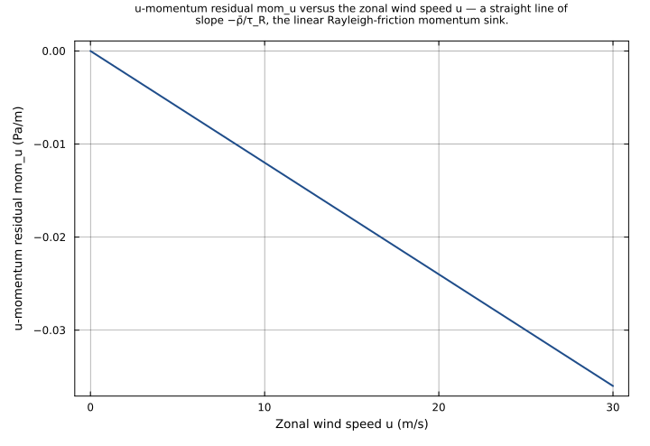
buoyancy_response
The w-momentum buoyancy term as a function of the density perturbation. The density perturbation ρ’ is swept from -0.1 to 0.1 kg/m³ with every other input at its default; the w-momentum residual reduces to mom_w = ρ’·g. Plotting mom_w against ρ’ gives a straight line of slope g = 9.81 m/s² — air denser than the base state (ρ’ > 0) produces a positive (downward-tending) residual, lighter air a negative one.
Time span: 0.0 → 1.0
Swept over: ρ_prime
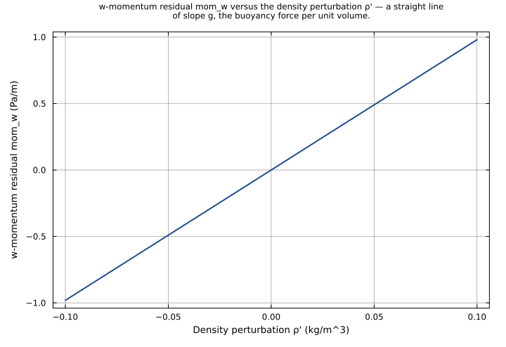
coriolis_friction_crossover
The crossover between the Coriolis term and the Rayleigh-friction sink in the u-momentum equation. The Rayleigh-friction time scale τ_R is swept logarithmically from 10 to 100000 s with a fixed zonal wind u = 10 m/s, ρ̄ = 1.2 kg/m³ and Coriolis parameter f = 1e-4 1/s, so mom_u = ρ̄·u·f − ρ̄·u/τ_R. For short τ_R the friction sink −ρ̄·u/τ_R dominates and mom_u is large and negative; as τ_R grows the friction term vanishes and mom_u approaches the Coriolis-only asymptote ρ̄·u·f = 0.0012 Pa/m. The plot shows this hyperbolic approach to the asymptote.
Time span: 0.0 → 1.0
Swept over: τ_R
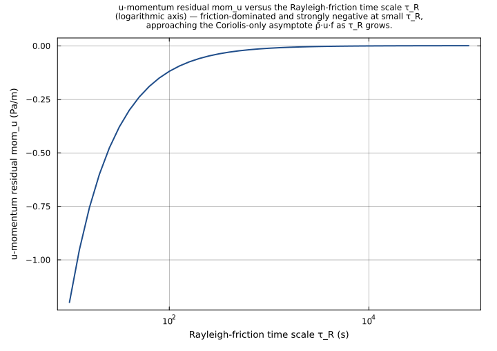
Raw .esm
Raw .esm JSON (this component)
{
"reference": {
"citation": "Clark, T. L. (1977). A Small-Scale Dynamic Model Using a Terrain-Following Coordinate Transformation. Journal of Computational Physics, 24(2), 186-215, Eqs. 2.1-2.3, 2.15.",
"notes": "source_ref: AtmosphericDynamics.jl@816cc3918e1eef2c2ee6d8fa8dd73c8f13a85a47:src/clark1977.jl:282\n\nUpstream `AnelasticMomentum` is an MTK `@component` returning `System(eqs, t; name)`. It textually declares 1 `@constants` (g) and 26 `@parameters` (u, v, w, du_dt, dv_dt, dw_dt, dp_dx, dp_dy, dp_dz, ρ, ρ_bar, ρ_prime, τ11, τ12, τ13, τ21, τ22, τ23, τ31, τ32, τ33, div_τ1, div_τ2, div_τ3, f_coriolis, τ_R), 3 `@variables` (mom_u, mom_v, mom_w) and 3 equations. Every equation is algebraic — there is no `D(...)` time derivative anywhere — so the component is a diagnostic momentum-residual evaluator: given the lowest-level dynamical state it returns, by direct substitution, the residual of each of the three Clark (1977) anelastic momentum equations.\n\nDead parameter declarations (10 of the 26 `@parameters` are intentionally not encoded). The equation set references only 16 of the 26 `@parameters` plus the constant g. The 10 unreferenced declarations — ρ (total density) and the nine Reynolds-stress-tensor components τ11, τ12, τ13, τ21, τ22, τ23, τ31, τ32, τ33 — never appear in any equation, so MTK's `System(eqs, t; name)` constructor (which collects variables and parameters from the equations) does not place them in `ModelingToolkit.parameters(sys)`: they are dead local bindings. The component takes the three stress divergences div_τ1/div_τ2/div_τ3 directly as inputs and never forms them from the individual τ_ij; and it uses the base-state density ρ̄ throughout (the upstream equation comments state 'using base-state density consistently'), never the total density ρ. The .esm therefore encodes exactly the 17 parameters that appear in `parameters(sys)` — g plus the 16 referenced `@parameters` — and omits the 10 dead declarations. This keeps the file self-consistent (every declared variable is referenced by an equation) and matches the system MTK actually builds. The same `parameters(sys)`-membership criterion governed the sibling surface_flux.esm migration.\n\nConstant treated as a parameter. The single MTK `@constants` (g) appears in `ModelingToolkit.parameters(sys)` alongside the `@parameters`, so it is encoded as `type: parameter`; the .esm schema has no dedicated constant variable type. This is the same treatment used by the sibling migrations surface_flux.esm (g, κ, V_min_sq, zero_Ri) and general_circulation.esm (Omega, R_earth, g).\n\nStructural shape (matches upstream test `AnelasticMomentum Structure`, test/clark1977_test.jl:218-223): `length(unknowns()) == 3`, `length(equations()) == 3`. The .esm preserves this exactly with 3 `type: state` variables and 3 entries in `equations`. All 3 `@variables` are encoded as `type: state` and carry no `default`: each is the LHS of one non-differential equation — an algebraic state determined by its equation, not initial-valued. After `mtkcompile` the upstream system moves all 3 to its `observed` set; the canonical Python runner resolves them directly, since each residual's right-hand side is a function of parameters only (no inter-state coupling).\n\nEquation set (matches src/clark1977.jl:338-347 verbatim):\n mom_u = ρ̄·du_dt + ρ̄·u·f_coriolis + dp_dx − div_τ1 − ρ̄·u/τ_R — Eq. 2.1, u-momentum residual: inertia + Coriolis + pressure-gradient force − Reynolds-stress divergence − Rayleigh friction.\n mom_v = ρ̄·dv_dt + ρ̄·v·f_coriolis + dp_dy − div_τ2 − ρ̄·v/τ_R — Eq. 2.2, v-momentum residual; identical structure to Eq. 2.1 with the y-direction inputs.\n mom_w = ρ̄·dw_dt + dp_dz + ρ'·g − div_τ3 − ρ̄·w/τ_R — Eq. 2.3, w-momentum residual: no Coriolis term in the vertical; the buoyancy term ρ'·g replaces it and uses the density perturbation ρ'.\nThe upstream Coriolis term is +ρ̄·u·f / +ρ̄·v·f (a velocity-aligned form, not the rotational −ρ̄·f·v / +ρ̄·f·u); the upstream equation comments label it 'Coriolis term is +ρ̃uf, using base-state density consistently'. It is migrated verbatim. The `+`, `*`, `/` ops are all first-class ESS expression ops (esm-schema.json ExpressionNode op enum); each subtraction is encoded as a `+` term scaled by −1.0, the negation convention used by the sibling surface_flux.esm.\n\nWell-posedness (no singularities): the only division is by τ_R, which has a default of 1000 s and is strictly positive in every test and example (smallest value used: 10 s, in the `coriolis_friction_crossover` example). Every residual is a finite closed-form polynomial/rational function of the parameters at every test point, so all inline tests are simulated directly — there is no 0/0 point to avoid.\n\nTolerance rationale (model-level rel=1e-6, abs=1e-9): a diagnostic algebraic system with no ODE integration — the assertion values are the closed-form evaluation of the upstream equations in IEEE-754 double precision. rel=1e-6 covers float64 round-off in the sums of products and the single division, and any sub-ULP difference between the Julia walker and the Python gate-of-record. abs=1e-9 covers the intended exact zeros — the residuals vanish identically under the default state (all velocities, derivatives, gradients and the density perturbation are zero) and under the `balanced_state` test (the pressure-gradient, stress-divergence and buoyancy terms cancel by construction), for which a pure relative bound is undefined. This rel/abs pair is the same one used by the sibling algebraic migrations surface_flux.esm and general_circulation.esm.\n\nUpstream test reproduction (test/clark1977_test.jl). The upstream Julia suite contains a single AnelasticMomentum test — `AnelasticMomentum Structure` (lines 218-223) — which only pins the structural counts (3 unknowns, 3 equations) and makes no numerical assertion. The .esm reproduces that structural check (3 `type: state` variables, 3 `equations`) and, per migration-guide §6.1, adds nine numerical tests that exercise all three equations term by term; each test pins all 3 residuals. Assertion values are the closed-form evaluation of the upstream equations:\n- `default_parameters` — all parameters at their declared defaults; every velocity, derivative, gradient, stress divergence and the density perturbation is zero, so all three residuals are exactly 0.\n- `inertial_acceleration` — isolates the inertial term ρ̄·(dV/dt) with nonzero material derivatives only, giving mom = ρ̄·(dV/dt).\n- `pressure_gradient` — isolates the pressure-gradient force with nonzero ∂p' gradients only, giving mom = ∂p'.\n- `buoyancy` — isolates the w-momentum buoyancy term with nonzero ρ' only, giving mom_w = ρ'·g and mom_u = mom_v = 0.\n- `stress_divergence` — isolates the Reynolds-stress divergence with nonzero div_τ only, giving mom = −div_τ.\n- `coriolis_and_friction` — nonzero horizontal velocities and Coriolis parameter; exercises the Coriolis term ρ̄·V·f together with the Rayleigh-friction sink ρ̄·V/τ_R (the two cannot be separated while V ≠ 0); mom_w = 0.\n- `rayleigh_friction` — nonzero velocities with f = 0; isolates the Rayleigh-friction sink mom = −ρ̄·V/τ_R in all three equations.\n- `full_momentum_residual` — every term active in all three equations; a combined non-trivial residual.\n- `balanced_state` — a physically meaningful case: the inputs are chosen so the pressure-gradient, stress-divergence and buoyancy terms cancel, driving every residual to zero — the 'exact solution' limit the upstream docstring describes ('Momentum equation residuals (should be zero for exact solution)').\n\nUnit balance (verified; no `checks=false` upstream): every term of every equation has the dimension of the residual, Pa/m = kg/(m²·s²). ρ̄·(dV/dt) = (kg/m³)·(m/s²) = kg/(m²·s²); ρ̄·V·f = (kg/m³)·(m/s)·(1/s) = kg/(m²·s²); ∂p' = Pa/m; div_τ = Pa/m; ρ'·g = (kg/m³)·(m/s²) = kg/(m²·s²); ρ̄·V/τ_R = (kg/m³)·(m/s)/s = kg/(m²·s²). SI throughout; no unit conversion at parse or runtime. The upstream component constructs its `System` without `checks=false`, so MTK's own dimensional analysis passes on these equations."
},
"tolerance": {
"rel": 1e-06,
"abs": 1e-09
},
"variables": {
"g": {
"type": "parameter",
"units": "m/s^2",
"default": 9.81,
"description": "Gravitational acceleration. Upstream MTK `@constants`; appears in the buoyancy term ρ'·g of the w-momentum equation (Eq. 2.3)."
},
"u": {
"type": "parameter",
"units": "m/s",
"default": 0.0,
"description": "x-velocity (zonal) component. Enters the Coriolis term ρ̄·u·f and the Rayleigh-friction sink ρ̄·u/τ_R of the u-momentum equation (Eq. 2.1)."
},
"v": {
"type": "parameter",
"units": "m/s",
"default": 0.0,
"description": "y-velocity (meridional) component. Enters the Coriolis term ρ̄·v·f and the Rayleigh-friction sink ρ̄·v/τ_R of the v-momentum equation (Eq. 2.2)."
},
"w": {
"type": "parameter",
"units": "m/s",
"default": 0.0,
"description": "z-velocity (vertical) component. Enters the Rayleigh-friction sink ρ̄·w/τ_R of the w-momentum equation (Eq. 2.3)."
},
"du_dt": {
"type": "parameter",
"units": "m/s^2",
"default": 0.0,
"description": "Material derivative of the x-velocity, du/dt. The inertial term ρ̄·(du/dt) of the u-momentum equation (Eq. 2.1)."
},
"dv_dt": {
"type": "parameter",
"units": "m/s^2",
"default": 0.0,
"description": "Material derivative of the y-velocity, dv/dt. The inertial term ρ̄·(dv/dt) of the v-momentum equation (Eq. 2.2)."
},
"dw_dt": {
"type": "parameter",
"units": "m/s^2",
"default": 0.0,
"description": "Material derivative of the z-velocity, dw/dt. The inertial term ρ̄·(dw/dt) of the w-momentum equation (Eq. 2.3)."
},
"dp_dx": {
"type": "parameter",
"units": "Pa/m",
"default": 0.0,
"description": "Perturbation-pressure gradient ∂p'/∂x — the x-component of the pressure-gradient force in the u-momentum equation (Eq. 2.1)."
},
"dp_dy": {
"type": "parameter",
"units": "Pa/m",
"default": 0.0,
"description": "Perturbation-pressure gradient ∂p'/∂y — the y-component of the pressure-gradient force in the v-momentum equation (Eq. 2.2)."
},
"dp_dz": {
"type": "parameter",
"units": "Pa/m",
"default": 0.0,
"description": "Perturbation-pressure gradient ∂p'/∂z — the z-component of the pressure-gradient force in the w-momentum equation (Eq. 2.3)."
},
"ρ_bar": {
"type": "parameter",
"units": "kg/m^3",
"default": 1.225,
"description": "Base-state (reference) air density ρ̄. Multiplies the inertial, Coriolis and Rayleigh-friction terms of all three momentum equations; the anelastic approximation uses the base-state density consistently."
},
"ρ_prime": {
"type": "parameter",
"units": "kg/m^3",
"default": 0.0,
"description": "Density perturbation ρ' from the base state. Drives the buoyancy term ρ'·g of the w-momentum equation (Eq. 2.3); a positive perturbation (air denser than the base state) contributes a positive residual."
},
"div_τ1": {
"type": "parameter",
"units": "Pa/m",
"default": 0.0,
"description": "Reynolds-stress divergence (∇·τ)₁ = ∂τ₁₁/∂x + ∂τ₁₂/∂y + ∂τ₁₃/∂z — the turbulent (subgrid) momentum flux entering the u-momentum equation (Eq. 2.1, stresses from Eq. 2.15)."
},
"div_τ2": {
"type": "parameter",
"units": "Pa/m",
"default": 0.0,
"description": "Reynolds-stress divergence (∇·τ)₂ = ∂τ₂₁/∂x + ∂τ₂₂/∂y + ∂τ₂₃/∂z — the turbulent (subgrid) momentum flux entering the v-momentum equation (Eq. 2.2, stresses from Eq. 2.15)."
},
"div_τ3": {
"type": "parameter",
"units": "Pa/m",
"default": 0.0,
"description": "Reynolds-stress divergence (∇·τ)₃ = ∂τ₃₁/∂x + ∂τ₃₂/∂y + ∂τ₃₃/∂z — the turbulent (subgrid) momentum flux entering the w-momentum equation (Eq. 2.3, stresses from Eq. 2.15)."
},
"f_coriolis": {
"type": "parameter",
"units": "1/s",
"default": 0.0,
"description": "Coriolis parameter f. Sets the magnitude of the Coriolis term ρ̄·V·f in the two horizontal momentum equations (Eqs. 2.1-2.2); there is no Coriolis term in the vertical."
},
"τ_R": {
"type": "parameter",
"units": "s",
"default": 1000.0,
"description": "Rayleigh-friction time scale. The momentum sink −ρ̄·V/τ_R in all three equations damps the velocity on the τ_R time scale (an absorbing-layer / large-scale-drag parameterization)."
},
"mom_u": {
"type": "unknown",
"units": "Pa/m",
"description": "u-momentum equation residual (Eq. 2.1): ρ̄·(du/dt) + ρ̄·u·f + ∂p'/∂x − (∇·τ)₁ − ρ̄·u/τ_R. Zero when the u-momentum balance is exactly satisfied."
},
"mom_v": {
"type": "unknown",
"units": "Pa/m",
"description": "v-momentum equation residual (Eq. 2.2): ρ̄·(dv/dt) + ρ̄·v·f + ∂p'/∂y − (∇·τ)₂ − ρ̄·v/τ_R. Zero when the v-momentum balance is exactly satisfied."
},
"mom_w": {
"type": "unknown",
"units": "Pa/m",
"description": "w-momentum equation residual (Eq. 2.3): ρ̄·(dw/dt) + ∂p'/∂z + ρ'·g − (∇·τ)₃ − ρ̄·w/τ_R. Zero when the w-momentum balance is exactly satisfied."
}
},
"equations": [
{
"_comment": "Eq. 2.1 — u-momentum equation residual: ρ̄·(du/dt) + ρ̄·u·f + ∂p'/∂x − (∇·τ)₁ − ρ̄·u/τ_R. Inertia + Coriolis + pressure-gradient force − Reynolds-stress divergence − Rayleigh friction; zero for an exact solution. The Coriolis term uses the base-state density ρ̄ consistently. Each subtraction is encoded as a term scaled by −1.0.",
"lhs": "mom_u",
"rhs": {
"op": "+",
"args": [
{
"op": "*",
"args": [
"ρ_bar",
"du_dt"
]
},
{
"op": "*",
"args": [
"ρ_bar",
"u",
"f_coriolis"
]
},
"dp_dx",
{
"op": "*",
"args": [
-1.0,
"div_τ1"
]
},
{
"op": "*",
"args": [
-1.0,
{
"op": "/",
"args": [
{
"op": "*",
"args": [
"ρ_bar",
"u"
]
},
"τ_R"
]
}
]
}
]
}
},
{
"_comment": "Eq. 2.2 — v-momentum equation residual: ρ̄·(dv/dt) + ρ̄·v·f + ∂p'/∂y − (∇·τ)₂ − ρ̄·v/τ_R. Identical structure to Eq. 2.1 with the y-direction inputs.",
"lhs": "mom_v",
"rhs": {
"op": "+",
"args": [
{
"op": "*",
"args": [
"ρ_bar",
"dv_dt"
]
},
{
"op": "*",
"args": [
"ρ_bar",
"v",
"f_coriolis"
]
},
"dp_dy",
{
"op": "*",
"args": [
-1.0,
"div_τ2"
]
},
{
"op": "*",
"args": [
-1.0,
{
"op": "/",
"args": [
{
"op": "*",
"args": [
"ρ_bar",
"v"
]
},
"τ_R"
]
}
]
}
]
}
},
{
"_comment": "Eq. 2.3 — w-momentum equation residual: ρ̄·(dw/dt) + ∂p'/∂z + ρ'·g − (∇·τ)₃ − ρ̄·w/τ_R. No Coriolis term in the vertical; the buoyancy term ρ'·g uses the density perturbation ρ'.",
"lhs": "mom_w",
"rhs": {
"op": "+",
"args": [
{
"op": "*",
"args": [
"ρ_bar",
"dw_dt"
]
},
"dp_dz",
{
"op": "*",
"args": [
"ρ_prime",
"g"
]
},
{
"op": "*",
"args": [
-1.0,
"div_τ3"
]
},
{
"op": "*",
"args": [
-1.0,
{
"op": "/",
"args": [
{
"op": "*",
"args": [
"ρ_bar",
"w"
]
},
"τ_R"
]
}
]
}
]
}
}
],
"tests": [
{
"id": "default_parameters",
"description": "All parameters at their declared defaults (every velocity, material derivative, pressure gradient, stress divergence, the Coriolis parameter and the density perturbation are zero; ρ_bar = 1.225, τ_R = 1000, g = 9.81). With no forcing of any kind every momentum-equation residual vanishes identically. Verifies the declared defaults are wired correctly. Pins all 3 variables.",
"parameter_overrides": {},
"time_span": {
"start": 0.0,
"end": 1.0
},
"assertions": [
{
"variable": "mom_u",
"time": 0.0,
"expected": 0.0
},
{
"variable": "mom_v",
"time": 0.0,
"expected": 0.0
},
{
"variable": "mom_w",
"time": 0.0,
"expected": 0.0
}
]
},
{
"id": "inertial_acceleration",
"description": "Isolates the inertial term ρ̄·(dV/dt). Only the material derivatives are nonzero (du/dt = 0.5, dv/dt = -0.25, dw/dt = 0.2 m/s²) with ρ̄ = 1.2 kg/m³; all velocities, gradients, stress divergences, Coriolis and density perturbation stay at zero, so each residual reduces to mom = ρ̄·(dV/dt). The Rayleigh-friction term is zero because the velocities are zero. Pins all 3 variables.",
"parameter_overrides": {
"ρ_bar": 1.2,
"du_dt": 0.5,
"dv_dt": -0.25,
"dw_dt": 0.2
},
"time_span": {
"start": 0.0,
"end": 1.0
},
"assertions": [
{
"variable": "mom_u",
"time": 0.0,
"expected": 0.6
},
{
"variable": "mom_v",
"time": 0.0,
"expected": -0.3
},
{
"variable": "mom_w",
"time": 0.0,
"expected": 0.24
}
]
},
{
"id": "pressure_gradient",
"description": "Isolates the perturbation-pressure-gradient force. Only the pressure gradients are nonzero (∂p'/∂x = 3.0, ∂p'/∂y = -2.5, ∂p'/∂z = -9.81 Pa/m); with every other input zero each residual reduces to mom = ∂p'. Pins all 3 variables.",
"parameter_overrides": {
"dp_dx": 3.0,
"dp_dy": -2.5,
"dp_dz": -9.81
},
"time_span": {
"start": 0.0,
"end": 1.0
},
"assertions": [
{
"variable": "mom_u",
"time": 0.0,
"expected": 3.0
},
{
"variable": "mom_v",
"time": 0.0,
"expected": -2.5
},
{
"variable": "mom_w",
"time": 0.0,
"expected": -9.81
}
]
},
{
"id": "buoyancy",
"description": "Isolates the w-momentum buoyancy term ρ'·g. Only the density perturbation is nonzero (ρ' = 0.05 kg/m³), so mom_w = ρ'·g = 0.05·9.81 and the two horizontal residuals stay zero (the buoyancy term appears only in the vertical equation). Pins all 3 variables.",
"parameter_overrides": {
"ρ_prime": 0.05
},
"time_span": {
"start": 0.0,
"end": 1.0
},
"assertions": [
{
"variable": "mom_u",
"time": 0.0,
"expected": 0.0
},
{
"variable": "mom_v",
"time": 0.0,
"expected": 0.0
},
{
"variable": "mom_w",
"time": 0.0,
"expected": 0.49050000000000005
}
]
},
{
"id": "stress_divergence",
"description": "Isolates the Reynolds-stress divergence. Only the stress divergences are nonzero ((∇·τ)₁ = 1.5, (∇·τ)₂ = -0.8, (∇·τ)₃ = 2.0 Pa/m); each residual reduces to mom = −div_τ — the stress divergence enters every momentum equation with a minus sign. Pins all 3 variables.",
"parameter_overrides": {
"div_τ1": 1.5,
"div_τ2": -0.8,
"div_τ3": 2.0
},
"time_span": {
"start": 0.0,
"end": 1.0
},
"assertions": [
{
"variable": "mom_u",
"time": 0.0,
"expected": -1.5
},
{
"variable": "mom_v",
"time": 0.0,
"expected": 0.8
},
{
"variable": "mom_w",
"time": 0.0,
"expected": -2.0
}
]
},
{
"id": "coriolis_and_friction",
"description": "Exercises the Coriolis term ρ̄·V·f together with the Rayleigh-friction sink ρ̄·V/τ_R. Nonzero horizontal velocities (u = 10, v = -5 m/s) with f = 1e-4 1/s, ρ̄ = 1.2 kg/m³ and τ_R = 2000 s: mom_u = ρ̄·u·f − ρ̄·u/τ_R and mom_v = ρ̄·v·f − ρ̄·v/τ_R (the two terms cannot be separated while V ≠ 0). The vertical residual is zero (w = 0). Pins all 3 variables.",
"parameter_overrides": {
"ρ_bar": 1.2,
"u": 10.0,
"v": -5.0,
"f_coriolis": 0.0001,
"τ_R": 2000.0
},
"time_span": {
"start": 0.0,
"end": 1.0
},
"assertions": [
{
"variable": "mom_u",
"time": 0.0,
"expected": -0.0048000000000000004
},
{
"variable": "mom_v",
"time": 0.0,
"expected": 0.0024000000000000002
},
{
"variable": "mom_w",
"time": 0.0,
"expected": 0.0
}
]
},
{
"id": "rayleigh_friction",
"description": "Isolates the Rayleigh-friction sink −ρ̄·V/τ_R in all three equations. Nonzero velocities (u = 8, v = 6, w = 2 m/s) with the Coriolis parameter f = 0, ρ̄ = 1.0 kg/m³ and τ_R = 1000 s: each residual reduces to mom = −ρ̄·V/τ_R, the linear momentum damping. Pins all 3 variables.",
"parameter_overrides": {
"ρ_bar": 1.0,
"u": 8.0,
"v": 6.0,
"w": 2.0,
"τ_R": 1000.0
},
"time_span": {
"start": 0.0,
"end": 1.0
},
"assertions": [
{
"variable": "mom_u",
"time": 0.0,
"expected": -0.008
},
{
"variable": "mom_v",
"time": 0.0,
"expected": -0.006
},
{
"variable": "mom_w",
"time": 0.0,
"expected": -0.002
}
]
},
{
"id": "full_momentum_residual",
"description": "Every term active in all three equations: ρ̄ = 1.0, ρ' = 0.1 kg/m³, u = 10, v = -6, w = 1 m/s, du/dt = 0.4, dv/dt = -0.2, dw/dt = 0.05 m/s², ∂p'/∂x = 1.0, ∂p'/∂y = -0.5, ∂p'/∂z = -9.0 Pa/m, (∇·τ)₁ = 0.2, (∇·τ)₂ = -0.3, (∇·τ)₃ = 0.5 Pa/m, f = 1e-4 1/s, τ_R = 1000 s. A combined non-trivial residual that exercises the inertial, Coriolis, pressure-gradient, stress-divergence, buoyancy and Rayleigh-friction terms simultaneously. Pins all 3 variables.",
"parameter_overrides": {
"ρ_bar": 1.0,
"ρ_prime": 0.1,
"u": 10.0,
"v": -6.0,
"w": 1.0,
"du_dt": 0.4,
"dv_dt": -0.2,
"dw_dt": 0.05,
"dp_dx": 1.0,
"dp_dy": -0.5,
"dp_dz": -9.0,
"div_τ1": 0.2,
"div_τ2": -0.3,
"div_τ3": 0.5,
"f_coriolis": 0.0001,
"τ_R": 1000.0
},
"time_span": {
"start": 0.0,
"end": 1.0
},
"assertions": [
{
"variable": "mom_u",
"time": 0.0,
"expected": 1.191
},
{
"variable": "mom_v",
"time": 0.0,
"expected": -0.3946
},
{
"variable": "mom_w",
"time": 0.0,
"expected": -8.469999999999999
}
]
},
{
"id": "balanced_state",
"description": "A physically meaningful case in which the momentum balance is exactly satisfied, so every residual vanishes. With all velocities and material derivatives zero, the u- and v-residuals reduce to ∂p' − div_τ; choosing ∂p'/∂x = (∇·τ)₁ = 0.7 and ∂p'/∂y = (∇·τ)₂ = -0.4 Pa/m cancels them. The w-residual reduces to ∂p'/∂z + ρ'·g; choosing ∂p'/∂z = -0.981 Pa/m against ρ' = 0.1 kg/m³ (ρ'·g = 0.1·9.81 = 0.981) cancels it. This is the 'exact solution' limit the upstream docstring describes. Pins all 3 variables.",
"parameter_overrides": {
"ρ_bar": 1.0,
"ρ_prime": 0.1,
"dp_dx": 0.7,
"dp_dy": -0.4,
"dp_dz": -0.981,
"div_τ1": 0.7,
"div_τ2": -0.4,
"div_τ3": 0.0
},
"time_span": {
"start": 0.0,
"end": 1.0
},
"assertions": [
{
"variable": "mom_u",
"time": 0.0,
"expected": 0.0
},
{
"variable": "mom_v",
"time": 0.0,
"expected": 0.0
},
{
"variable": "mom_w",
"time": 0.0,
"expected": 0.0
}
]
}
],
"analyses": [
{
"id": "rayleigh_friction_response",
"description": "The Rayleigh-friction momentum sink as a function of wind speed. The zonal velocity u is swept from 0 to 30 m/s with ρ̄ = 1.2 kg/m³ and τ_R = 1000 s; every other input is left at its zero default, so the u-momentum residual reduces to mom_u = −ρ̄·u/τ_R. Plotting mom_u against u shows the linear momentum damping — the absorbing-layer / large-scale-drag term removes momentum in proportion to the wind speed.",
"initial_state": {},
"parameters": {
"ρ_bar": 1.2,
"τ_R": 1000.0
},
"time_span": {
"start": 0.0,
"end": 1.0
},
"parameter_sweep": {
"type": "cartesian",
"dimensions": [
{
"parameter": "u",
"range": {
"start": 0.0,
"stop": 30.0,
"count": 31,
"scale": "linear"
}
}
]
},
"plots": [
{
"id": "momu_vs_wind",
"type": "line",
"description": "u-momentum residual mom_u versus the zonal wind speed u — a straight line of slope −ρ̄/τ_R, the linear Rayleigh-friction momentum sink.",
"x": {
"variable": "u",
"label": "Zonal wind speed u (m/s)"
},
"y": {
"variable": "mom_u",
"label": "u-momentum residual mom_u (Pa/m)"
}
}
]
},
{
"id": "buoyancy_response",
"description": "The w-momentum buoyancy term as a function of the density perturbation. The density perturbation ρ' is swept from -0.1 to 0.1 kg/m³ with every other input at its default; the w-momentum residual reduces to mom_w = ρ'·g. Plotting mom_w against ρ' gives a straight line of slope g = 9.81 m/s² — air denser than the base state (ρ' > 0) produces a positive (downward-tending) residual, lighter air a negative one.",
"initial_state": {},
"parameters": {},
"time_span": {
"start": 0.0,
"end": 1.0
},
"parameter_sweep": {
"type": "cartesian",
"dimensions": [
{
"parameter": "ρ_prime",
"range": {
"start": -0.1,
"stop": 0.1,
"count": 41,
"scale": "linear"
}
}
]
},
"plots": [
{
"id": "momw_vs_rhoprime",
"type": "line",
"description": "w-momentum residual mom_w versus the density perturbation ρ' — a straight line of slope g, the buoyancy force per unit volume.",
"x": {
"variable": "ρ_prime",
"label": "Density perturbation ρ' (kg/m^3)"
},
"y": {
"variable": "mom_w",
"label": "w-momentum residual mom_w (Pa/m)"
}
}
]
},
{
"id": "coriolis_friction_crossover",
"description": "The crossover between the Coriolis term and the Rayleigh-friction sink in the u-momentum equation. The Rayleigh-friction time scale τ_R is swept logarithmically from 10 to 100000 s with a fixed zonal wind u = 10 m/s, ρ̄ = 1.2 kg/m³ and Coriolis parameter f = 1e-4 1/s, so mom_u = ρ̄·u·f − ρ̄·u/τ_R. For short τ_R the friction sink −ρ̄·u/τ_R dominates and mom_u is large and negative; as τ_R grows the friction term vanishes and mom_u approaches the Coriolis-only asymptote ρ̄·u·f = 0.0012 Pa/m. The plot shows this hyperbolic approach to the asymptote.",
"initial_state": {},
"parameters": {
"ρ_bar": 1.2,
"u": 10.0,
"f_coriolis": 0.0001
},
"time_span": {
"start": 0.0,
"end": 1.0
},
"parameter_sweep": {
"type": "cartesian",
"dimensions": [
{
"parameter": "τ_R",
"range": {
"start": 10.0,
"stop": 100000.0,
"count": 41,
"scale": "log"
}
}
]
},
"plots": [
{
"id": "momu_vs_tauR",
"type": "line",
"description": "u-momentum residual mom_u versus the Rayleigh-friction time scale τ_R (logarithmic axis) — friction-dominated and strongly negative at small τ_R, approaching the Coriolis-only asymptote ρ̄·u·f as τ_R grows.",
"x": {
"variable": "τ_R",
"label": "Rayleigh-friction time scale τ_R (s)"
},
"y": {
"variable": "mom_u",
"label": "u-momentum residual mom_u (Pa/m)"
}
}
]
}
]
}