ParticleCollectionEfficiency
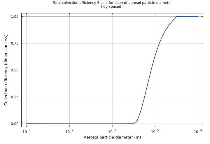
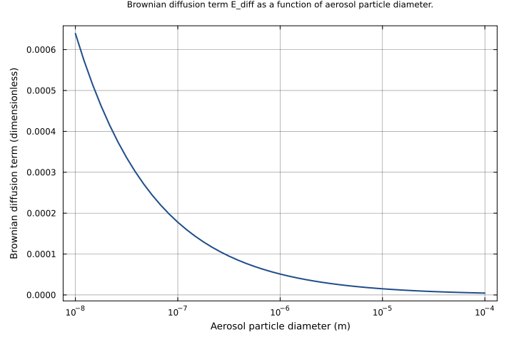
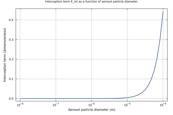
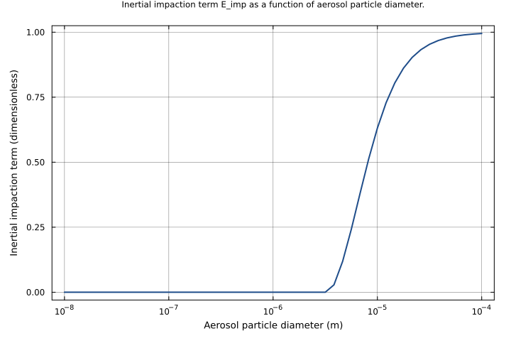
Slinn (1983) semi-empirical collision (collection) efficiency E between a falling raindrop and an aerosol particle, the kernel of below-cloud particle scavenging (Eqs. 20.53-20.54, Seinfeld & Pandis, 2006). E is the sum of three collection mechanisms — Brownian diffusion (E_diff, important for sub-0.1 µm particles), interception (E_int), and inertial impaction (E_imp, important for super-µm particles, switched on only when the Stokes number exceeds the critical Stokes number S* of Eq. 20.54) — and is clamped to a maximum of 1. The competition between the diffusion and impaction mechanisms produces the Greenfield gap: a collection-efficiency minimum at accumulation-mode (~0.1-1 µm) particle sizes. Migrated from AtmosphericDeposition.jl@e4468c79 src/seinfeld_pandis_2006_ch20.jl:365 (`ParticleCollectionEfficiency` @component). The upstream component carries the single equation E ~ slinn_collection_efficiency(D_p, U_t, d_p, ρ_p, T); the helper function and its sub-helpers (particle_diffusivity, particle_relaxation_time, particle_terminal_velocity) are decomposed here into 18 named intermediate algebraic states (Re, D_diff, Sc, τ, St, S_star, E_diff, E_int, E_imp, ...) mirroring the helper's local variables, so each equation maps to one source line. Observed-only: all 18 equations are algebraic — the five raindrop/aerosol/thermodynamic inputs and six physical constants are parameters, and Re through E are the algebraic outputs.
Description
Slinn (1983) semi-empirical collision (collection) efficiency E between a falling raindrop and an aerosol particle, the kernel of below-cloud particle scavenging (Eqs. 20.53-20.54, Seinfeld & Pandis, 2006). E is the sum of three collection mechanisms — Brownian diffusion (E_diff, important for sub-0.1 µm particles), interception (E_int), and inertial impaction (E_imp, important for super-µm particles, switched on only when the Stokes number exceeds the critical Stokes number S* of Eq. 20.54) — and is clamped to a maximum of 1. The competition between the diffusion and impaction mechanisms produces the Greenfield gap: a collection-efficiency minimum at accumulation-mode (~0.1-1 µm) particle sizes. Migrated from AtmosphericDeposition.jl@e4468c79 src/seinfeld_pandis_2006_ch20.jl:365 (ParticleCollectionEfficiency @component). The upstream component carries the single equation E ~ slinn_collection_efficiency(D_p, U_t, d_p, ρ_p, T); the helper function and its sub-helpers (particle_diffusivity, particle_relaxation_time, particle_terminal_velocity) are decomposed here into 18 named intermediate algebraic states (Re, D_diff, Sc, τ, St, S_star, E_diff, E_int, E_imp, …) mirroring the helper’s local variables, so each equation maps to one source line. Observed-only: all 18 equations are algebraic — the five raindrop/aerosol/thermodynamic inputs and six physical constants are parameters, and Re through E are the algebraic outputs.
Reference
_source_ref: AtmosphericDeposition.jl@e4468c79c8dd4aae88646cd16d6bcf290874742c:src/seinfeld_pandis_2006_ch20.jl:365
Upstream ParticleCollectionEfficiency is an MTK @component with D_p, U_t, d_p, ρ_p, T as input @parameters and a single output @variable E(t), related by one equation E ~ slinn_collection_efficiency(D_p, U_t, d_p, ρ_p, T) — the Slinn (1983) semi-empirical raindrop-aerosol collision (collection) efficiency, Seinfeld & Pandis (2006) Eqs. 20.53-20.54. It returns System(eqs, t, vars, params; name) with no subsystems, so it is a flat algebraic model.
Decomposition: the upstream slinn_collection_efficiency is a module-level helper function whose result is one large symbolic expression. Inlining it verbatim into a single equation AST would duplicate the Re / Sc / St / S_star / stokes_diff / safe_ratio subexpressions many times over (Re alone is referenced ~6 times, stokes_diff ~5), producing a several-hundred-node tree that is not reviewable. Instead the helper’s named local variables are migrated as 18 intermediate algebraic states — one equation each, in the helper’s own evaluation order — so every .esm equation maps to exactly one source line and the migration is line-checkable. This is mathematically identical to the single upstream equation (the intermediates are common-subexpression names); after mtkcompile all 18 reduce to observed quantities and E is the same function of the five inputs as upstream. The three module-level sub-helpers particle_diffusivity (Stokes-Einstein, src line 290), particle_relaxation_time (src line 268) and particle_terminal_velocity (src line 278) are inlined into the D_diff, τ and u_t_particle equations respectively. This extends the sibling air_refreshing.esm / cloud_ice_uptake.esm convention of inlining upstream helper functions, with named intermediates because this component’s single helper is far larger than those siblings'.
The six module-level @constants (μ_air_sp, ρ_air_sp, μ_w_sp, ρ_w_sp, g_sp, kB_sp) migrate as fixed-default type: parameter entries holding their upstream numeric values (Seinfeld & Pandis 2006; μ_air from Table A.7), per the rig convention for translating MTK @constants (matches cloud_ice_uptake.esm). The upstream cbrt(Sc) cube root in the Brownian term is re-expressed as Sc^(1/3) with the ^ op, since the spec §4.2 elementary-function set has no cbrt; Sc (a Schmidt number) is always strictly positive so the two are numerically equivalent. Julia’s pi is inlined as the float64 literal 3.141592653589793. The upstream 1//12 and 2//3 exact rationals are kept as integer-literal / nodes. The component has no ifelse nodes: the upstream final clamp ifelse(E_total > 1, 1, E_total) is migrated as min(1, E_total) — the identical upper clamp and the spec §4.2-preferred AST encoding of a limiter — and the upstream impaction term ifelse(stokes_diff ≤ 0, zero(safe_ratio), safe_ratiosqrt(safe_ratio)) is migrated as safe_ratiosqrt(safe_ratio) directly, because safe_ratio = max(0, stokes_diff)/(max(0, stokes_diff) + 2/3) is already exactly 0 whenever stokes_diff ≤ 0 (the max(0, ·) numerator), so both ifelse branches are bit-identical and the conditional is provably dead code. Eliding it is numerically exact and keeps the model free of Piecewise: a Max reachable from a Piecewise condition trips a sympy lambdify-printer path (simplify_logic substitutes every free symbol with 0, and the resulting 0/0 in the zeroed Reynolds/Stokes expressions reaches Max as a NaN). The max(0, ·) in safe_ratio is retained — it keeps the sqrt argument non-negative, the upstream author’s own stated reason for the max (‘avoid negative base in power’). system_kind is left unset (zero differential states — no D operator), consistent with the observed-only siblings air_refreshing.esm / atmospheric_thermo.esm / total_molar_conc.esm.
The five input parameters carry their upstream @parameter defaults (D_p = 1e-3 m, U_t = 4 m/s, d_p = 1e-6 m, ρ_p = 1000 kg/m^3, T = 298 K). Upstream provides three relevant test items: Slinn Collection Efficiency (Eq. 20.53) exercises the helper at small / medium / large aerosol diameters with inequality assertions (E_small > 1e-4, E_small > E_medium, all E ≤ 1); Critical Stokes Number (Eq. 20.54) checks the S* formula; and the helper-function items pin particle_relaxation_time ≈ 3.23e-6 s, particle_terminal_velocity ≈ 3.17e-5 m/s and particle_diffusivity ≈ 2.54e-11 m^2/s at d_p = 1e-6 m, ρ_p = 1000 kg/m^3, T = 298 K. The inline tests here pin exact values: default_parameters uses the component defaults (which coincide with the upstream helper-test inputs) and asserts τ, u_t_particle and D_diff against those upstream reference values plus the full chain; aitken_mode_aerosol / accumulation_mode_aerosol / coarse_mode_aerosol reproduce the upstream Slinn Collection Efficiency small / medium / large cases (D_p = 2e-3 m, U_t = 6.5 m/s, d_p ∈ {1e-8, 1e-6, 1e-5} m) and confirm E_small > E_medium and the Greenfield-gap minimum at accumulation-mode size; coarse_mode_aerosol and dense_coarse_aerosol exercise the St > S* inertial-impaction branch and the sqrt(ρ_w/ρ_p) density correction; cold_temperature exercises the temperature dependence of the Brownian term; efficiency_clamp drives E_total > 1 so the Eq. 20.53 maximum-of-1 clamp fires (E pinned to 1.0).
Tolerance rationale (model-level rel=1e-6, abs=1e-12): observed-only algebraic system (no ODE integration). The 18 equations form a triangular chain of +, -, *, /, ^, sqrt, log, max and min on float64; round-off is ~1e-16 per op, so rel=1e-6 leaves ample headroom across the tested ranges (Re ~ 1e2, Sc ~ 5e3 to 3e7, E ~ 1e-4 to 1). abs=1e-12 gates the exact-zero intermediates (safe_ratio, E_imp_unscaled, E_imp) in the no-impaction cases, where a pure relative tolerance would be degenerate._
Parameters
| Name | Units | Default | Description |
|---|---|---|---|
D_p | m | 0.001 | Raindrop diameter |
U_t | m/s | 4.0 | Terminal velocity of the raindrop |
d_p | m | 1e-06 | Aerosol particle diameter |
ρ_p | kg/m^3 | 1000.0 | Aerosol particle density |
T | K | 298.0 | Temperature |
μ_air_sp | kg/(m*s) | 1.72e-05 | Dynamic viscosity of air (Table A.7, Seinfeld & Pandis 2006) |
ρ_air_sp | kg/m^3 | 1.225 | Air density at standard conditions (Seinfeld & Pandis 2006) |
μ_w_sp | kg/(m*s) | 0.001 | Dynamic viscosity of water |
ρ_w_sp | kg/m^3 | 1000.0 | Water density |
g_sp | m/s^2 | 9.81 | Gravitational acceleration |
kB_sp | kg*m^2/(s^2*K) | 1.3806488e-23 | Boltzmann constant |
Observed
| Name | Units | Default | Description |
|---|---|---|---|
Re | 1 | Raindrop Reynolds number based on drop radius, Re = D_pU_tρ_air/(2*μ_air) (dimensionless) | |
D_diff | m^2/s | Brownian diffusivity of the aerosol particle (Stokes-Einstein relation) | |
Sc | 1 | Particle Schmidt number, Sc = μ_air/(ρ_air*D_diff) (dimensionless) | |
τ | s | Particle relaxation time in the Stokes drag regime, τ = ρ_pd_p^2/(18μ_air) | |
u_t_particle | m/s | Particle Stokes settling (terminal) velocity, u_t = τ*g | |
St | 1 | Stokes number of the aerosol particle relative to the raindrop, St = 2τ(U_t - u_t)/D_p (dimensionless) | |
φ | 1 | Aerosol-to-raindrop diameter ratio, φ = d_p/D_p (dimensionless) | |
ω | 1 | Water-to-air dynamic viscosity ratio, ω = μ_w/μ_air (dimensionless) | |
S_star | 1 | Critical Stokes number (Eq. 20.54) (dimensionless) | |
E_diff | 1 | Brownian diffusion term of the collection efficiency (Eq. 20.53, first line) (dimensionless) | |
E_int | 1 | Interception term of the collection efficiency (Eq. 20.53, second line) (dimensionless) | |
stokes_diff | 1 | Stokes-number excess over the critical Stokes number, St - S* (dimensionless) | |
safe_ratio | 1 | Clamped impaction ratio max(0, St-S*)/(max(0, St-S*) + 2/3) (dimensionless) | |
density_scaling | 1 | Particle-density correction factor sqrt(ρ_w/ρ_p) for the impaction term (dimensionless) | |
E_imp_unscaled | 1 | Inertial impaction term before the density correction; zero when St ≤ S* (dimensionless) | |
E_imp | 1 | Inertial impaction term of the collection efficiency (Eq. 20.53, third line) (dimensionless) | |
E_total | 1 | Sum of the three collection-efficiency terms before clamping (dimensionless) | |
E | 1 | Collection efficiency between a raindrop and an aerosol particle (Eq. 20.53), clamped to a maximum of 1 (dimensionless) |
Observed expressions
$$ Re = \frac{D_{p} \cdot U_{t} \cdot ρ_{air\,sp}}{2 \cdot μ_{air\,sp}} $$Raindrop Reynolds number based on drop radius, Re = D_pU_tρ_air/(2*μ_air) (dimensionless)
$$ D_{diff} = \frac{kB_{sp} \cdot T}{3 \cdot 3.141592653589793 \cdot μ_{air\,sp} \cdot d_{p}} $$Brownian diffusivity of the aerosol particle (Stokes-Einstein relation)
$$ Sc = \frac{μ_{air\,sp}}{ρ_{air\,sp} \cdot D_{diff}} $$Particle Schmidt number, Sc = μ_air/(ρ_air*D_diff) (dimensionless)
$$ τ = \frac{ρ_{p} \cdot d_{p}^{2}}{18 \cdot μ_{air\,sp}} $$Particle relaxation time in the Stokes drag regime, τ = ρ_pd_p^2/(18μ_air)
$$ u_{t\,particle} = τ \cdot g_{sp} $$Particle Stokes settling (terminal) velocity, u_t = τ*g
$$ St = \frac{2 \cdot τ \cdot \left(U_{t} - u_{t\,particle}\right)}{D_{p}} $$Stokes number of the aerosol particle relative to the raindrop, St = 2τ(U_t - u_t)/D_p (dimensionless)
$$ φ = \frac{d_{p}}{D_{p}} $$Aerosol-to-raindrop diameter ratio, φ = d_p/D_p (dimensionless)
$$ ω = \frac{μ_{w\,sp}}{μ_{air\,sp}} $$Water-to-air dynamic viscosity ratio, ω = μ_w/μ_air (dimensionless)
$$ S_{star} = \frac{1.2 + \frac{1}{12} \cdot \ln\left(1 + Re\right)}{1 + \ln\left(1 + Re\right)} $$Critical Stokes number (Eq. 20.54) (dimensionless)
$$ E_{diff} = \frac{4}{Re \cdot Sc} \cdot \left(1 + 0.4 \cdot \sqrt{Re} \cdot Sc^{\frac{1}{3}} + 0.16 \cdot \sqrt{Re} \cdot \sqrt{Sc}\right) $$Brownian diffusion term of the collection efficiency (Eq. 20.53, first line) (dimensionless)
$$ E_{int} = 4 \cdot φ \cdot \left(\frac{1}{ω} + \left(1 + 2 \cdot \sqrt{Re}\right) \cdot φ\right) $$Interception term of the collection efficiency (Eq. 20.53, second line) (dimensionless)
$$ stokes_{diff} = St - S_{star} $$Stokes-number excess over the critical Stokes number, St - S* (dimensionless)
$$ safe_{ratio} = \frac{\mathrm{max}\left(0, stokes_{diff}\right)}{\mathrm{max}\left(0, stokes_{diff}\right) + \frac{2}{3}} $$Clamped impaction ratio max(0, St-S*)/(max(0, St-S*) + 2/3) (dimensionless)
$$ density_{scaling} = \sqrt{\frac{ρ_{w\,sp}}{ρ_{p}}} $$Particle-density correction factor sqrt(ρ_w/ρ_p) for the impaction term (dimensionless)
$$ E_{imp\,unscaled} = safe_{ratio} \cdot \sqrt{safe_{ratio}} $$Inertial impaction term before the density correction; zero when St ≤ S* (dimensionless)
$$ E_{imp} = E_{imp\,unscaled} \cdot density_{scaling} $$Inertial impaction term of the collection efficiency (Eq. 20.53, third line) (dimensionless)
$$ E_{total} = E_{diff} + E_{int} + E_{imp} $$Sum of the three collection-efficiency terms before clamping (dimensionless)
$$ E = \mathrm{min}\left(1, E_{total}\right) $$Collection efficiency between a raindrop and an aerosol particle (Eq. 20.53), clamped to a maximum of 1 (dimensionless)
Analyses
collection_efficiency_vs_aerosol_size
Slinn (1983) collection efficiency and its three mechanisms as a function of aerosol particle diameter, for a 2 mm raindrop falling at 6.5 m/s. This reproduces the canonical below-cloud scavenging figure (Seinfeld & Pandis 2006, Fig. 20.13): Brownian diffusion dominates for d_p below ~0.1 µm, inertial impaction dominates above ~1 µm, and the two leave a minimum — the Greenfield gap — at accumulation-mode sizes.
Time span: 0.0 → 1.0
Swept over: d_p
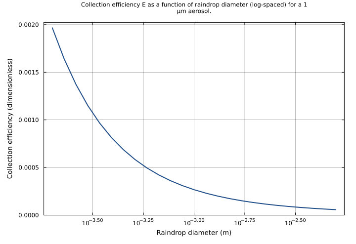
collection_efficiency_vs_raindrop_size
Collection efficiency of a 1 µm accumulation-mode aerosol as a function of raindrop diameter, at a fixed fall speed U_t = 6.5 m/s. Smaller raindrops are more efficient collectors per drop (the interception and Brownian terms scale inversely with raindrop size), so E falls as the raindrop diameter grows.
Time span: 0.0 → 1.0
Swept over: D_p
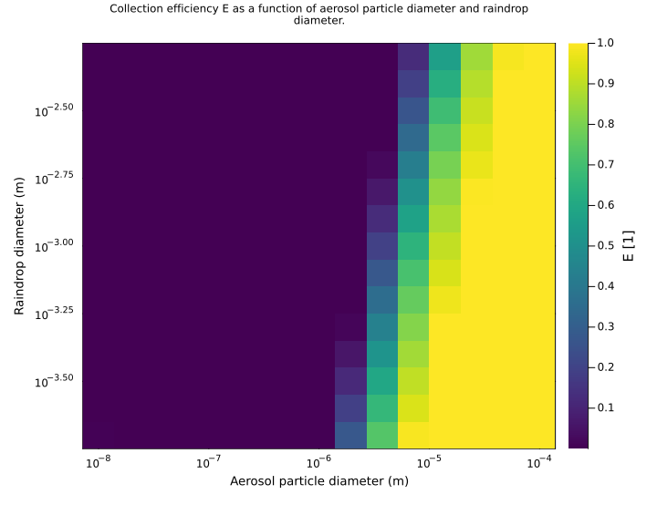
efficiency_over_aerosol_and_raindrop_size
Two-dimensional sweep of the collection efficiency E over aerosol particle diameter (10 nm to 100 µm, log-spaced) and raindrop diameter (0.2 mm to 5 mm, log-spaced) at a fixed fall speed U_t = 6.5 m/s. Surfaces the joint control of particle and raindrop size on below-cloud particle scavenging efficiency.
Time span: 0.0 → 1.0
Swept over: d_p, D_p
Raw .esm
Raw .esm JSON (this component)
{
"reference": {
"notes": "source_ref: AtmosphericDeposition.jl@e4468c79c8dd4aae88646cd16d6bcf290874742c:src/seinfeld_pandis_2006_ch20.jl:365\nUpstream `ParticleCollectionEfficiency` is an MTK `@component` with D_p, U_t, d_p, ρ_p, T as input `@parameters` and a single output `@variable` E(t), related by one equation E ~ slinn_collection_efficiency(D_p, U_t, d_p, ρ_p, T) — the Slinn (1983) semi-empirical raindrop-aerosol collision (collection) efficiency, Seinfeld & Pandis (2006) Eqs. 20.53-20.54. It returns `System(eqs, t, vars, params; name)` with no subsystems, so it is a flat algebraic model.\n\nDecomposition: the upstream `slinn_collection_efficiency` is a module-level helper function whose result is one large symbolic expression. Inlining it verbatim into a single equation AST would duplicate the Re / Sc / St / S_star / stokes_diff / safe_ratio subexpressions many times over (Re alone is referenced ~6 times, stokes_diff ~5), producing a several-hundred-node tree that is not reviewable. Instead the helper's named local variables are migrated as 18 intermediate algebraic states — one equation each, in the helper's own evaluation order — so every .esm equation maps to exactly one source line and the migration is line-checkable. This is mathematically identical to the single upstream equation (the intermediates are common-subexpression names); after `mtkcompile` all 18 reduce to observed quantities and E is the same function of the five inputs as upstream. The three module-level sub-helpers `particle_diffusivity` (Stokes-Einstein, src line 290), `particle_relaxation_time` (src line 268) and `particle_terminal_velocity` (src line 278) are inlined into the D_diff, τ and u_t_particle equations respectively. This extends the sibling air_refreshing.esm / cloud_ice_uptake.esm convention of inlining upstream helper functions, with named intermediates because this component's single helper is far larger than those siblings'.\n\nThe six module-level `@constants` (μ_air_sp, ρ_air_sp, μ_w_sp, ρ_w_sp, g_sp, kB_sp) migrate as fixed-default `type: parameter` entries holding their upstream numeric values (Seinfeld & Pandis 2006; μ_air from Table A.7), per the rig convention for translating MTK `@constants` (matches cloud_ice_uptake.esm). The upstream `cbrt(Sc)` cube root in the Brownian term is re-expressed as Sc^(1/3) with the `^` op, since the spec §4.2 elementary-function set has no `cbrt`; Sc (a Schmidt number) is always strictly positive so the two are numerically equivalent. Julia's `pi` is inlined as the float64 literal 3.141592653589793. The upstream `1//12` and `2//3` exact rationals are kept as integer-literal `/` nodes. The component has no `ifelse` nodes: the upstream final clamp ifelse(E_total > 1, 1, E_total) is migrated as min(1, E_total) — the identical upper clamp and the spec §4.2-preferred AST encoding of a limiter — and the upstream impaction term ifelse(stokes_diff ≤ 0, zero(safe_ratio), safe_ratio*sqrt(safe_ratio)) is migrated as safe_ratio*sqrt(safe_ratio) directly, because safe_ratio = max(0, stokes_diff)/(max(0, stokes_diff) + 2/3) is already exactly 0 whenever stokes_diff ≤ 0 (the max(0, ·) numerator), so both ifelse branches are bit-identical and the conditional is provably dead code. Eliding it is numerically exact and keeps the model free of `Piecewise`: a `Max` reachable from a `Piecewise` condition trips a sympy lambdify-printer path (`simplify_logic` substitutes every free symbol with 0, and the resulting 0/0 in the zeroed Reynolds/Stokes expressions reaches `Max` as a NaN). The max(0, ·) in safe_ratio is retained — it keeps the sqrt argument non-negative, the upstream author's own stated reason for the max ('avoid negative base in power'). `system_kind` is left unset (zero differential states — no D operator), consistent with the observed-only siblings air_refreshing.esm / atmospheric_thermo.esm / total_molar_conc.esm.\n\nThe five input parameters carry their upstream `@parameter` defaults (D_p = 1e-3 m, U_t = 4 m/s, d_p = 1e-6 m, ρ_p = 1000 kg/m^3, T = 298 K). Upstream provides three relevant test items: `Slinn Collection Efficiency (Eq. 20.53)` exercises the helper at small / medium / large aerosol diameters with inequality assertions (E_small > 1e-4, E_small > E_medium, all E ≤ 1); `Critical Stokes Number (Eq. 20.54)` checks the S* formula; and the helper-function items pin particle_relaxation_time ≈ 3.23e-6 s, particle_terminal_velocity ≈ 3.17e-5 m/s and particle_diffusivity ≈ 2.54e-11 m^2/s at d_p = 1e-6 m, ρ_p = 1000 kg/m^3, T = 298 K. The inline tests here pin exact values: default_parameters uses the component defaults (which coincide with the upstream helper-test inputs) and asserts τ, u_t_particle and D_diff against those upstream reference values plus the full chain; aitken_mode_aerosol / accumulation_mode_aerosol / coarse_mode_aerosol reproduce the upstream `Slinn Collection Efficiency` small / medium / large cases (D_p = 2e-3 m, U_t = 6.5 m/s, d_p ∈ {1e-8, 1e-6, 1e-5} m) and confirm E_small > E_medium and the Greenfield-gap minimum at accumulation-mode size; coarse_mode_aerosol and dense_coarse_aerosol exercise the St > S* inertial-impaction branch and the sqrt(ρ_w/ρ_p) density correction; cold_temperature exercises the temperature dependence of the Brownian term; efficiency_clamp drives E_total > 1 so the Eq. 20.53 maximum-of-1 clamp fires (E pinned to 1.0).\n\nTolerance rationale (model-level rel=1e-6, abs=1e-12): observed-only algebraic system (no ODE integration). The 18 equations form a triangular chain of +, -, *, /, ^, sqrt, log, max and min on float64; round-off is ~1e-16 per op, so rel=1e-6 leaves ample headroom across the tested ranges (Re ~ 1e2, Sc ~ 5e3 to 3e7, E ~ 1e-4 to 1). abs=1e-12 gates the exact-zero intermediates (safe_ratio, E_imp_unscaled, E_imp) in the no-impaction cases, where a pure relative tolerance would be degenerate."
},
"tolerance": {
"rel": 1e-06,
"abs": 1e-12
},
"variables": {
"D_p": {
"type": "parameter",
"units": "m",
"default": 0.001,
"description": "Raindrop diameter"
},
"U_t": {
"type": "parameter",
"units": "m/s",
"default": 4.0,
"description": "Terminal velocity of the raindrop"
},
"d_p": {
"type": "parameter",
"units": "m",
"default": 1e-06,
"description": "Aerosol particle diameter"
},
"ρ_p": {
"type": "parameter",
"units": "kg/m^3",
"default": 1000.0,
"description": "Aerosol particle density"
},
"T": {
"type": "parameter",
"units": "K",
"default": 298.0,
"description": "Temperature"
},
"μ_air_sp": {
"type": "parameter",
"units": "kg/(m*s)",
"default": 1.72e-05,
"description": "Dynamic viscosity of air (Table A.7, Seinfeld & Pandis 2006)"
},
"ρ_air_sp": {
"type": "parameter",
"units": "kg/m^3",
"default": 1.225,
"description": "Air density at standard conditions (Seinfeld & Pandis 2006)"
},
"μ_w_sp": {
"type": "parameter",
"units": "kg/(m*s)",
"default": 0.001,
"description": "Dynamic viscosity of water"
},
"ρ_w_sp": {
"type": "parameter",
"units": "kg/m^3",
"default": 1000.0,
"description": "Water density"
},
"g_sp": {
"type": "parameter",
"units": "m/s^2",
"default": 9.81,
"description": "Gravitational acceleration"
},
"kB_sp": {
"type": "parameter",
"units": "kg*m^2/(s^2*K)",
"default": 1.3806488e-23,
"description": "Boltzmann constant"
},
"Re": {
"type": "unknown",
"units": "1",
"description": "Raindrop Reynolds number based on drop radius, Re = D_p*U_t*ρ_air/(2*μ_air) (dimensionless)"
},
"D_diff": {
"type": "unknown",
"units": "m^2/s",
"description": "Brownian diffusivity of the aerosol particle (Stokes-Einstein relation)"
},
"Sc": {
"type": "unknown",
"units": "1",
"description": "Particle Schmidt number, Sc = μ_air/(ρ_air*D_diff) (dimensionless)"
},
"τ": {
"type": "unknown",
"units": "s",
"description": "Particle relaxation time in the Stokes drag regime, τ = ρ_p*d_p^2/(18*μ_air)"
},
"u_t_particle": {
"type": "unknown",
"units": "m/s",
"description": "Particle Stokes settling (terminal) velocity, u_t = τ*g"
},
"St": {
"type": "unknown",
"units": "1",
"description": "Stokes number of the aerosol particle relative to the raindrop, St = 2*τ*(U_t - u_t)/D_p (dimensionless)"
},
"φ": {
"type": "unknown",
"units": "1",
"description": "Aerosol-to-raindrop diameter ratio, φ = d_p/D_p (dimensionless)"
},
"ω": {
"type": "unknown",
"units": "1",
"description": "Water-to-air dynamic viscosity ratio, ω = μ_w/μ_air (dimensionless)"
},
"S_star": {
"type": "unknown",
"units": "1",
"description": "Critical Stokes number (Eq. 20.54) (dimensionless)"
},
"E_diff": {
"type": "unknown",
"units": "1",
"description": "Brownian diffusion term of the collection efficiency (Eq. 20.53, first line) (dimensionless)"
},
"E_int": {
"type": "unknown",
"units": "1",
"description": "Interception term of the collection efficiency (Eq. 20.53, second line) (dimensionless)"
},
"stokes_diff": {
"type": "unknown",
"units": "1",
"description": "Stokes-number excess over the critical Stokes number, St - S* (dimensionless)"
},
"safe_ratio": {
"type": "unknown",
"units": "1",
"description": "Clamped impaction ratio max(0, St-S*)/(max(0, St-S*) + 2/3) (dimensionless)"
},
"density_scaling": {
"type": "unknown",
"units": "1",
"description": "Particle-density correction factor sqrt(ρ_w/ρ_p) for the impaction term (dimensionless)"
},
"E_imp_unscaled": {
"type": "unknown",
"units": "1",
"description": "Inertial impaction term before the density correction; zero when St ≤ S* (dimensionless)"
},
"E_imp": {
"type": "unknown",
"units": "1",
"description": "Inertial impaction term of the collection efficiency (Eq. 20.53, third line) (dimensionless)"
},
"E_total": {
"type": "unknown",
"units": "1",
"description": "Sum of the three collection-efficiency terms before clamping (dimensionless)"
},
"E": {
"type": "unknown",
"units": "1",
"description": "Collection efficiency between a raindrop and an aerosol particle (Eq. 20.53), clamped to a maximum of 1 (dimensionless)"
}
},
"equations": [
{
"_comment": "Reynolds number based on drop radius (slinn_collection_efficiency, src line 310): Re = D_p*U_t*ρ_air/(2*μ_air)",
"lhs": "Re",
"rhs": {
"op": "/",
"args": [
{
"op": "*",
"args": [
"D_p",
"U_t",
"ρ_air_sp"
]
},
{
"op": "*",
"args": [
2,
"μ_air_sp"
]
}
]
}
},
{
"_comment": "Brownian diffusivity of the aerosol particle via Stokes-Einstein (particle_diffusivity, src line 291): D_diff = k_B*T/(3*pi*μ_air*d_p)",
"lhs": "D_diff",
"rhs": {
"op": "/",
"args": [
{
"op": "*",
"args": [
"kB_sp",
"T"
]
},
{
"op": "*",
"args": [
3,
3.141592653589793,
"μ_air_sp",
"d_p"
]
}
]
}
},
{
"_comment": "Particle Schmidt number (slinn_collection_efficiency, src line 314): Sc = μ_air/(ρ_air*D_diff)",
"lhs": "Sc",
"rhs": {
"op": "/",
"args": [
"μ_air_sp",
{
"op": "*",
"args": [
"ρ_air_sp",
"D_diff"
]
}
]
}
},
{
"_comment": "Particle relaxation time in the Stokes drag regime (particle_relaxation_time, src line 269): τ = ρ_p*d_p^2/(18*μ_air)",
"lhs": "τ",
"rhs": {
"op": "/",
"args": [
{
"op": "*",
"args": [
"ρ_p",
{
"op": "^",
"args": [
"d_p",
2
]
}
]
},
{
"op": "*",
"args": [
18,
"μ_air_sp"
]
}
]
}
},
{
"_comment": "Particle Stokes settling velocity (particle_terminal_velocity, src line 280): u_t = τ*g",
"lhs": "u_t_particle",
"rhs": {
"op": "*",
"args": [
"τ",
"g_sp"
]
}
},
{
"_comment": "Stokes number of the aerosol particle relative to the raindrop (slinn_collection_efficiency, src line 319): St = 2*τ*(U_t - u_t)/D_p",
"lhs": "St",
"rhs": {
"op": "/",
"args": [
{
"op": "*",
"args": [
2,
"τ",
{
"op": "-",
"args": [
"U_t",
"u_t_particle"
]
}
]
},
"D_p"
]
}
},
{
"_comment": "Aerosol-to-raindrop diameter ratio (slinn_collection_efficiency, src line 322): φ = d_p/D_p",
"lhs": "φ",
"rhs": {
"op": "/",
"args": [
"d_p",
"D_p"
]
}
},
{
"_comment": "Water-to-air dynamic viscosity ratio (slinn_collection_efficiency, src line 325): ω = μ_w/μ_air",
"lhs": "ω",
"rhs": {
"op": "/",
"args": [
"μ_w_sp",
"μ_air_sp"
]
}
},
{
"_comment": "Critical Stokes number (Eq. 20.54; slinn_collection_efficiency, src line 328): S* = (1.2 + (1/12)*log(1+Re))/(1 + log(1+Re))",
"lhs": "S_star",
"rhs": {
"op": "/",
"args": [
{
"op": "+",
"args": [
1.2,
{
"op": "*",
"args": [
{
"op": "/",
"args": [
1,
12
]
},
{
"op": "log",
"args": [
{
"op": "+",
"args": [
1,
"Re"
]
}
]
}
]
}
]
},
{
"op": "+",
"args": [
1,
{
"op": "log",
"args": [
{
"op": "+",
"args": [
1,
"Re"
]
}
]
}
]
}
]
}
},
{
"_comment": "Brownian diffusion term of the collection efficiency (Eq. 20.53, first line; slinn_collection_efficiency, src line 331): E_diff = (4/(Re*Sc))*(1 + 0.4*sqrt(Re)*Sc^(1/3) + 0.16*sqrt(Re)*sqrt(Sc)). The upstream cbrt(Sc) is re-expressed as Sc^(1/3) (no cbrt op in spec §4.2); Sc > 0 always, so the two are equivalent.",
"lhs": "E_diff",
"rhs": {
"op": "*",
"args": [
{
"op": "/",
"args": [
4,
{
"op": "*",
"args": [
"Re",
"Sc"
]
}
]
},
{
"op": "+",
"args": [
1,
{
"op": "*",
"args": [
0.4,
{
"op": "sqrt",
"args": [
"Re"
]
},
{
"op": "^",
"args": [
"Sc",
{
"op": "/",
"args": [
1,
3
]
}
]
}
]
},
{
"op": "*",
"args": [
0.16,
{
"op": "sqrt",
"args": [
"Re"
]
},
{
"op": "sqrt",
"args": [
"Sc"
]
}
]
}
]
}
]
}
},
{
"_comment": "Interception term of the collection efficiency (Eq. 20.53, second line; slinn_collection_efficiency, src line 334): E_int = 4*φ*(1/ω + (1 + 2*sqrt(Re))*φ)",
"lhs": "E_int",
"rhs": {
"op": "*",
"args": [
4,
"φ",
{
"op": "+",
"args": [
{
"op": "/",
"args": [
1,
"ω"
]
},
{
"op": "*",
"args": [
{
"op": "+",
"args": [
1,
{
"op": "*",
"args": [
2,
{
"op": "sqrt",
"args": [
"Re"
]
}
]
}
]
},
"φ"
]
}
]
}
]
}
},
{
"_comment": "Stokes-number excess over the critical Stokes number (slinn_collection_efficiency, src line 342): stokes_diff = St - S*",
"lhs": "stokes_diff",
"rhs": {
"op": "-",
"args": [
"St",
"S_star"
]
}
},
{
"_comment": "Clamped impaction ratio (slinn_collection_efficiency, src line 344): max(0, St-S*)/(max(0, St-S*) + 2/3). The max(0, ·) keeps safe_ratio non-negative so the downstream sqrt(safe_ratio) in E_imp_unscaled is real-valued, and makes safe_ratio exactly 0 when St ≤ S*.",
"lhs": "safe_ratio",
"rhs": {
"op": "/",
"args": [
{
"op": "max",
"args": [
0,
"stokes_diff"
]
},
{
"op": "+",
"args": [
{
"op": "max",
"args": [
0,
"stokes_diff"
]
},
{
"op": "/",
"args": [
2,
3
]
}
]
}
]
}
},
{
"_comment": "Particle-density correction factor for the impaction term (slinn_collection_efficiency, src line 345; Seinfeld & Pandis p. 950): density_scaling = sqrt(ρ_w/ρ_p)",
"lhs": "density_scaling",
"rhs": {
"op": "sqrt",
"args": [
{
"op": "/",
"args": [
"ρ_w_sp",
"ρ_p"
]
}
]
}
},
{
"_comment": "Inertial impaction term before the density correction (slinn_collection_efficiency, src line 347): safe_ratio*sqrt(safe_ratio) = safe_ratio^(3/2). Upstream wraps this in ifelse(St-S* ≤ 0, 0, safe_ratio*sqrt(safe_ratio)) so the term is zero when St ≤ S* (impaction requires sufficient inertia; Seinfeld & Pandis p. 950); the ifelse is omitted because safe_ratio = max(0, St-S*)/(max(0, St-S*) + 2/3) is already exactly 0 when St-S* ≤ 0, so both ifelse branches are bit-identical.",
"lhs": "E_imp_unscaled",
"rhs": {
"op": "*",
"args": [
"safe_ratio",
{
"op": "sqrt",
"args": [
"safe_ratio"
]
}
]
}
},
{
"_comment": "Inertial impaction term of the collection efficiency (Eq. 20.53, third line; slinn_collection_efficiency, src line 351): E_imp = E_imp_unscaled*density_scaling",
"lhs": "E_imp",
"rhs": {
"op": "*",
"args": [
"E_imp_unscaled",
"density_scaling"
]
}
},
{
"_comment": "Sum of the three collection-efficiency mechanisms before clamping (slinn_collection_efficiency, src line 353): E_total = E_diff + E_int + E_imp",
"lhs": "E_total",
"rhs": {
"op": "+",
"args": [
"E_diff",
"E_int",
"E_imp"
]
}
},
{
"_comment": "Collection efficiency clamped to a maximum of 1 (Eq. 20.53; slinn_collection_efficiency, src line 355): E = min(1, E_total). Upstream writes ifelse(E_total > 1, 1, E_total); min(1, E_total) is the identical upper clamp and the spec §4.2-preferred AST encoding of a clamp/limiter.",
"lhs": "E",
"rhs": {
"op": "min",
"args": [
1,
"E_total"
]
}
}
],
"tests": [
{
"id": "default_parameters",
"description": "Component defaults (D_p = 1 mm raindrop, U_t = 4 m/s, d_p = 1 µm accumulation-mode aerosol, ρ_p = 1000 kg/m^3, T = 298 K). These inputs coincide with the upstream helper-function test inputs, so τ, u_t_particle, and D_diff are pinned against the upstream reference values (particle_relaxation_time ≈ 3.23e-6 s, particle_terminal_velocity ≈ 3.17e-5 m/s, particle_diffusivity ≈ 2.54e-11 m^2/s). The Stokes number St ≈ 0.026 falls below the critical S* ≈ 0.27, so the impaction term is off and E is the sum of the small Brownian and interception terms. The system is algebraic, so E is re-asserted at t = 1 to confirm time-invariance.",
"parameter_overrides": {
"D_p": 0.001,
"U_t": 4.0,
"d_p": 1e-06,
"ρ_p": 1000.0,
"T": 298.0
},
"time_span": {
"start": 0.0,
"end": 1.0
},
"assertions": [
{
"variable": "Re",
"time": 0.0,
"expected": 142.4418604651163
},
{
"variable": "D_diff",
"time": 0.0,
"expected": 2.5380484572007868e-11
},
{
"variable": "Sc",
"time": 0.0,
"expected": 553213.0912116716
},
{
"variable": "τ",
"time": 0.0,
"expected": 3.2299741602067182e-06
},
{
"variable": "u_t_particle",
"time": 0.0,
"expected": 3.168604651162791e-05
},
{
"variable": "St",
"time": 0.0,
"expected": 0.025839588591430804
},
{
"variable": "φ",
"time": 0.0,
"expected": 0.001
},
{
"variable": "ω",
"time": 0.0,
"expected": 58.13953488372093
},
{
"variable": "S_star",
"time": 0.0,
"expected": 0.2705072867967095
},
{
"variable": "E_diff",
"time": 0.0,
"expected": 9.204065626656528e-05
},
{
"variable": "E_int",
"time": 0.0,
"expected": 0.0001682792075258663
},
{
"variable": "E_imp",
"time": 0.0,
"expected": 0.0
},
{
"variable": "E",
"time": 0.0,
"expected": 0.0002603198637924316
},
{
"variable": "E",
"time": 1.0,
"expected": 0.0002603198637924316
}
]
},
{
"id": "aitken_mode_aerosol",
"description": "Small Aitken-mode aerosol (d_p = 10 nm) collected by a 2 mm raindrop falling at 6.5 m/s — the upstream `Slinn Collection Efficiency` small-particle case. Brownian diffusion dominates (E_diff ≫ E_int); the Stokes number is far below S* so the impaction term is zero. This is the high-efficiency small-particle end of the Slinn curve, with E larger than the accumulation-mode case (upstream assertion E_small > E_medium).",
"parameter_overrides": {
"D_p": 0.002,
"U_t": 6.5,
"d_p": 1e-08,
"ρ_p": 1000.0,
"T": 298.0
},
"time_span": {
"start": 0.0,
"end": 1.0
},
"assertions": [
{
"variable": "Re",
"time": 0.0,
"expected": 462.9360465116279
},
{
"variable": "E_diff",
"time": 0.0,
"expected": 0.000639219579960086
},
{
"variable": "E_int",
"time": 0.0,
"expected": 3.4840318973093977e-07
},
{
"variable": "E_imp",
"time": 0.0,
"expected": 0.0
},
{
"variable": "E",
"time": 0.0,
"expected": 0.0006395679831498169
}
]
},
{
"id": "accumulation_mode_aerosol",
"description": "Accumulation-mode aerosol (d_p = 1 µm) collected by a 2 mm raindrop falling at 6.5 m/s — the upstream `Slinn Collection Efficiency` medium-particle case. This is the Greenfield gap: Brownian diffusion has weakened and inertial impaction has not yet switched on, so the collection efficiency E is at its minimum — smaller than both the aitken_mode_aerosol and coarse_mode_aerosol cases at the same raindrop.",
"parameter_overrides": {
"D_p": 0.002,
"U_t": 6.5,
"d_p": 1e-06,
"ρ_p": 1000.0,
"T": 298.0
},
"time_span": {
"start": 0.0,
"end": 1.0
},
"assertions": [
{
"variable": "E_diff",
"time": 0.0,
"expected": 5.104243173195447e-05
},
{
"variable": "E_int",
"time": 0.0,
"expected": 7.843189730939726e-05
},
{
"variable": "E",
"time": 0.0,
"expected": 0.00012947432904135173
}
]
},
{
"id": "coarse_mode_aerosol",
"description": "Coarse-mode aerosol (d_p = 10 µm) collected by a 2 mm raindrop falling at 6.5 m/s — the upstream `Slinn Collection Efficiency` large-particle case. The Stokes number St ≈ 2.1 now exceeds the critical S* ≈ 0.24, so the inertial impaction term switches on (stokes_diff > 0) and dominates E. With ρ_p = ρ_w the density correction sqrt(ρ_w/ρ_p) = 1, so E_imp = E_imp_unscaled.",
"parameter_overrides": {
"D_p": 0.002,
"U_t": 6.5,
"d_p": 1e-05,
"ρ_p": 1000.0,
"T": 298.0
},
"time_span": {
"start": 0.0,
"end": 1.0
},
"assertions": [
{
"variable": "St",
"time": 0.0,
"expected": 2.0984597530196507
},
{
"variable": "S_star",
"time": 0.0,
"expected": 0.23973477328922943
},
{
"variable": "stokes_diff",
"time": 0.0,
"expected": 1.8587249797304213
},
{
"variable": "safe_ratio",
"time": 0.0,
"expected": 0.7360145434797082
},
{
"variable": "density_scaling",
"time": 0.0,
"expected": 1.0
},
{
"variable": "E_imp_unscaled",
"time": 0.0,
"expected": 0.6314363712214995
},
{
"variable": "E_imp",
"time": 0.0,
"expected": 0.6314363712214995
},
{
"variable": "E_int",
"time": 0.0,
"expected": 0.004747189730939727
},
{
"variable": "E",
"time": 0.0,
"expected": 0.636198586474696
}
]
},
{
"id": "dense_coarse_aerosol",
"description": "Dense coarse-mode aerosol (d_p = 10 µm, ρ_p = 2000 kg/m^3 — roughly mineral dust) collected by a 2 mm raindrop at 6.5 m/s. The doubled density doubles the relaxation time τ and hence the Stokes number relative to coarse_mode_aerosol, raising the unscaled impaction term, but the density correction sqrt(ρ_w/ρ_p) = sqrt(0.5) ≈ 0.707 scales the impaction term back down — exercising the ρ_p ≠ ρ_w branch of the density correction.",
"parameter_overrides": {
"D_p": 0.002,
"U_t": 6.5,
"d_p": 1e-05,
"ρ_p": 2000.0,
"T": 298.0
},
"time_span": {
"start": 0.0,
"end": 1.0
},
"assertions": [
{
"variable": "τ",
"time": 0.0,
"expected": 0.0006459948320413437
},
{
"variable": "St",
"time": 0.0,
"expected": 4.194872603809867
},
{
"variable": "stokes_diff",
"time": 0.0,
"expected": 3.9551378305206377
},
{
"variable": "safe_ratio",
"time": 0.0,
"expected": 0.8557561949943185
},
{
"variable": "density_scaling",
"time": 0.0,
"expected": 0.7071067811865476
},
{
"variable": "E_imp_unscaled",
"time": 0.0,
"expected": 0.7916351650323278
},
{
"variable": "E_imp",
"time": 0.0,
"expected": 0.5597705934200907
},
{
"variable": "E",
"time": 0.0,
"expected": 0.5645328086732871
}
]
},
{
"id": "cold_temperature",
"description": "Component defaults but at a cold T = 273 K. Brownian diffusivity scales linearly with temperature (Stokes-Einstein), so the colder column has a smaller D_diff and a larger Schmidt number Sc than the 298 K default_parameters case, which lowers the Brownian diffusion term E_diff. The interception and impaction terms are temperature-independent.",
"parameter_overrides": {
"D_p": 0.001,
"U_t": 4.0,
"d_p": 1e-06,
"ρ_p": 1000.0,
"T": 273.0
},
"time_span": {
"start": 0.0,
"end": 1.0
},
"assertions": [
{
"variable": "D_diff",
"time": 0.0,
"expected": 2.3251249289121297e-11
},
{
"variable": "Sc",
"time": 0.0,
"expected": 603873.6306999201
},
{
"variable": "E_diff",
"time": 0.0,
"expected": 8.78172093972164e-05
},
{
"variable": "E",
"time": 0.0,
"expected": 0.0002560964169230827
}
]
},
{
"id": "efficiency_clamp",
"description": "Large light aerosol (d_p = 50 µm, ρ_p = 500 kg/m^3) collected by a 2 mm raindrop at 6.5 m/s. The large relaxation time gives a Stokes number St ≈ 26, and the density correction sqrt(ρ_w/ρ_p) = sqrt(2) ≈ 1.414 amplifies the impaction term so that the unclamped sum E_total ≈ 1.47 exceeds 1. The Eq. 20.53 maximum-of-1 clamp therefore fires and E is pinned to exactly 1.0 — exercising the E_total > 1 branch.",
"parameter_overrides": {
"D_p": 0.002,
"U_t": 6.5,
"d_p": 5e-05,
"ρ_p": 500.0,
"T": 298.0
},
"time_span": {
"start": 0.0,
"end": 1.0
},
"assertions": [
{
"variable": "E_imp",
"time": 0.0,
"expected": 1.3612050562639566
},
{
"variable": "E_total",
"time": 0.0,
"expected": 1.4730112686254653
},
{
"variable": "E",
"time": 0.0,
"expected": 1.0
}
]
}
],
"analyses": [
{
"id": "collection_efficiency_vs_aerosol_size",
"description": "Slinn (1983) collection efficiency and its three mechanisms as a function of aerosol particle diameter, for a 2 mm raindrop falling at 6.5 m/s. This reproduces the canonical below-cloud scavenging figure (Seinfeld & Pandis 2006, Fig. 20.13): Brownian diffusion dominates for d_p below ~0.1 µm, inertial impaction dominates above ~1 µm, and the two leave a minimum — the Greenfield gap — at accumulation-mode sizes.",
"initial_state": {},
"parameters": {
"D_p": 0.002,
"U_t": 6.5,
"ρ_p": 1000.0,
"T": 298.0
},
"time_span": {
"start": 0.0,
"end": 1.0
},
"parameter_sweep": {
"type": "cartesian",
"dimensions": [
{
"parameter": "d_p",
"range": {
"start": 1e-08,
"stop": 0.0001,
"count": 49,
"scale": "log"
}
}
]
},
"plots": [
{
"id": "E_vs_dp",
"type": "line",
"description": "Total collection efficiency E as a function of aerosol particle diameter (log-spaced).",
"x": {
"variable": "d_p",
"label": "Aerosol particle diameter (m)"
},
"y": {
"variable": "E",
"label": "Collection efficiency (dimensionless)"
}
},
{
"id": "E_diff_vs_dp",
"type": "line",
"description": "Brownian diffusion term E_diff as a function of aerosol particle diameter.",
"x": {
"variable": "d_p",
"label": "Aerosol particle diameter (m)"
},
"y": {
"variable": "E_diff",
"label": "Brownian diffusion term (dimensionless)"
}
},
{
"id": "E_int_vs_dp",
"type": "line",
"description": "Interception term E_int as a function of aerosol particle diameter.",
"x": {
"variable": "d_p",
"label": "Aerosol particle diameter (m)"
},
"y": {
"variable": "E_int",
"label": "Interception term (dimensionless)"
}
},
{
"id": "E_imp_vs_dp",
"type": "line",
"description": "Inertial impaction term E_imp as a function of aerosol particle diameter.",
"x": {
"variable": "d_p",
"label": "Aerosol particle diameter (m)"
},
"y": {
"variable": "E_imp",
"label": "Inertial impaction term (dimensionless)"
}
}
]
},
{
"id": "collection_efficiency_vs_raindrop_size",
"description": "Collection efficiency of a 1 µm accumulation-mode aerosol as a function of raindrop diameter, at a fixed fall speed U_t = 6.5 m/s. Smaller raindrops are more efficient collectors per drop (the interception and Brownian terms scale inversely with raindrop size), so E falls as the raindrop diameter grows.",
"initial_state": {},
"parameters": {
"U_t": 6.5,
"d_p": 1e-06,
"ρ_p": 1000.0,
"T": 298.0
},
"time_span": {
"start": 0.0,
"end": 1.0
},
"parameter_sweep": {
"type": "cartesian",
"dimensions": [
{
"parameter": "D_p",
"range": {
"start": 0.0002,
"stop": 0.005,
"count": 25,
"scale": "log"
}
}
]
},
"plots": [
{
"id": "E_vs_Dp",
"type": "line",
"description": "Collection efficiency E as a function of raindrop diameter (log-spaced) for a 1 µm aerosol.",
"x": {
"variable": "D_p",
"label": "Raindrop diameter (m)"
},
"y": {
"variable": "E",
"label": "Collection efficiency (dimensionless)"
}
}
]
},
{
"id": "efficiency_over_aerosol_and_raindrop_size",
"description": "Two-dimensional sweep of the collection efficiency E over aerosol particle diameter (10 nm to 100 µm, log-spaced) and raindrop diameter (0.2 mm to 5 mm, log-spaced) at a fixed fall speed U_t = 6.5 m/s. Surfaces the joint control of particle and raindrop size on below-cloud particle scavenging efficiency.",
"initial_state": {},
"parameters": {
"U_t": 6.5,
"ρ_p": 1000.0,
"T": 298.0
},
"time_span": {
"start": 0.0,
"end": 1.0
},
"parameter_sweep": {
"type": "cartesian",
"dimensions": [
{
"parameter": "d_p",
"range": {
"start": 1e-08,
"stop": 0.0001,
"count": 15,
"scale": "log"
}
},
{
"parameter": "D_p",
"range": {
"start": 0.0002,
"stop": 0.005,
"count": 15,
"scale": "log"
}
}
]
},
"plots": [
{
"id": "E_heatmap",
"type": "heatmap",
"description": "Collection efficiency E as a function of aerosol particle diameter and raindrop diameter.",
"x": {
"variable": "d_p",
"label": "Aerosol particle diameter (m)"
},
"y": {
"variable": "D_p",
"label": "Raindrop diameter (m)"
},
"value": {
"variable": "E",
"reduce": "final"
}
}
]
}
]
}