ReactionTimescale
ModelingToolkit implementation of the characteristic timescale for aqueous-phase chemical reaction within a cloud droplet or wetted aerosol particle, from Seinfeld & Pandis (2006), Atmospheric Chemistry and Physics, 2nd ed., Chapter 12, Eqs. 12.76-12.78. The component reports two diagnostics for a first-order aqueous reaction: the aqueous-phase reaction timescale τ_ra = 1/k_rxn (Eq. 12.76), the e-folding time of a dissolved species consumed by a first-order reaction of rate constant k_rxn; and the gas-phase reference reaction timescale τ_rg = τ_ra/(H*·R·T) (Eq. 12.78), the same timescale referenced to the gas phase through the dimensionless effective Henry's law solubility H*·R·T. Migrated from Aerosol.jl ReactionTimescale. Purely algebraic: no differential states, two observed outputs and an empty equations array.
Description
ModelingToolkit implementation of the characteristic timescale for aqueous-phase chemical reaction within a cloud droplet or wetted aerosol particle, from Seinfeld & Pandis (2006), Atmospheric Chemistry and Physics, 2nd ed., Chapter 12, Eqs. 12.76-12.78. The component reports two diagnostics for a first-order aqueous reaction: the aqueous-phase reaction timescale τ_ra = 1/k_rxn (Eq. 12.76), the e-folding time of a dissolved species consumed by a first-order reaction of rate constant k_rxn; and the gas-phase reference reaction timescale τ_rg = τ_ra/(H*·R·T) (Eq. 12.78), the same timescale referenced to the gas phase through the dimensionless effective Henry’s law solubility H*·R·T. Migrated from Aerosol.jl ReactionTimescale. Purely algebraic: no differential states, two observed outputs and an empty equations array.
Reference
Seinfeld, J. H., and Pandis, S. N. (2006). Atmospheric Chemistry and Physics: From Air Pollution to Climate Change, 2nd Edition, John Wiley & Sons, Chapter 12. Aqueous-phase reaction timescale: Eq. 12.76; gas-phase reference reaction timescale: Eq. 12.78.
_source_ref: Aerosol.jl@c8c640bb636b22f2425460e9ed5cba50793bfee1:src/timescales.jl:110
Upstream ReactionTimescale is an MTK @component with one @constants entry (R, the universal gas constant), three @parameters (k_rxn, H_star, T), two time-indexed @variables (τ_ra, τ_rg), and two equations:
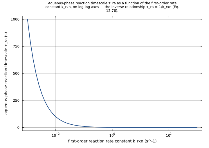
• Eq. 12.76: τ_ra ~ 1 / k_rxn — aqueous-phase reaction timescale of a first-order reaction
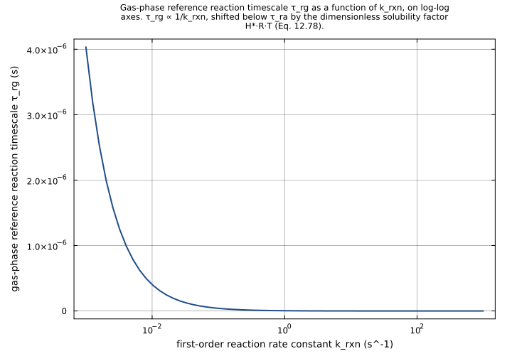
• Eq. 12.78: τ_rg ~ τ_ra / (H_star * R * T) — gas-phase reference reaction timescale
Both equations are algebraic (a plain lhs ~ rhs with no D(·) time derivative); the component has no differential state anywhere.
Observability classification: observed-only. With no differential state, MTK mtkcompile/structural_simplify reduces the raw 2-unknown / 2-equation System(eqs, t) to zero ODE states plus two observed quantities recovered algebraically. τ_ra and τ_rg are therefore encoded as type: observed, each carrying its defining relation in its expression field, and the equations array is empty — the post-mtkcompile representation, matching the migration-tracker features: ...observed classification and sibling observed-only components critical_ssa.esm and mean_free_path.esm. τ_rg’s expression references the observed variable τ_ra by name, preserving the upstream equation symbol-for-symbol; the canonical ESS runner resolves the observed-to-observed dependency, as it does in sibling tropospheric_budget.esm (observed tau_total referencing observed k_total).
Constant handling: the upstream @constants R = 8.314 migrates as a type: parameter with a fixed default — the ESS schema has no constant variable type, so every @constant becomes a fixed-default parameter (the convention sibling mean_free_path.esm applies to its R/M_air/π_val constants). R is one of the three reserved physical-constant names in the ESS schema (R, k_B, N_A); it is declared here with units J/(mol*K), dimensionally compatible with the canonical ideal-gas-constant dimension, so it passes the schema’s physical-constant unit check (parse.py _check_physical_constant_units).
Tests: the upstream component carries no test suite (migration-tracker has_tests: N). The seven inline tests below are authored directly from the two analytic formulas — τ_ra = 1/k_rxn and τ_rg = (1/k_rxn)/(H_star·R·T) — evaluated in float64 at the declared defaults or a single-parameter override. Because both outputs are algebraic and time-independent, default_conditions asserts at both t=0 and t=1 to confirm time-invariance; the remaining tests assert at t=0. Coverage sweeps the reaction rate constant (fast/slow first-order reaction), the effective Henry’s law solubility (high/low), and the temperature (cold/warm); every test also pins τ_ra to confirm it is independent of H_star and T.
Tolerance rationale (model-level rel=1e-9): observed-only algebraic system, no ODE integration. τ_ra is a single division and τ_rg is a three-factor product followed by a division; float64 round-off is ~1e-15, so rel=1e-9 leaves six orders of magnitude of headroom and absorbs any associativity difference in the n-ary product H_star·R·T. The pinned expected values are the exact analytic formulas, so the migration is checkable against the textbook equations, not merely against a prior solver run.
Unit balance (verified):
τ_ra 1 / k_rxn: 1/(s^-1) = s
τ_rg τ_ra / (H_star * R * T): s / (mol/(m^3Pa) · J/(molK) · K) = s / (J/(m^3*Pa)); since J = Pa·m^3 the product H_star·R·T = (Pa·m^3)/(m^3·Pa) = 1 (the dimensionless effective Henry’s law solubility), so τ_rg = s / 1 = s
SI throughout; no unit conversion at parse or runtime._
Parameters
| Name | Units | Default | Description |
|---|---|---|---|
R | J/(mol*K) | 8.314 | Universal (ideal) gas constant. Carried as a fixed-default parameter because the ESS schema has no constant variable type; the upstream value is the MTK @constant R = 8.314 J/(mol*K). |
k_rxn | s^-1 | 1.0 | First-order rate constant of the aqueous-phase chemical reaction consuming the dissolved species. Sets the aqueous-phase reaction timescale τ_ra = 1/k_rxn. |
H_star | mol/(m^3*Pa) | 100000.0 | Effective Henry’s law coefficient of the species — the equilibrium ratio of dissolved (aqueous) to gas-phase abundance, enhanced where aqueous-phase dissociation or reaction increases the apparent solubility. Enters the dimensionless solubility factor H*·R·T. |
T | K | 298.15 | Absolute temperature. |
Observed
| Name | Units | Default | Description |
|---|---|---|---|
τ_ra | s | Aqueous-phase reaction timescale (Seinfeld & Pandis 2006, Eq. 12.76): the e-folding time τ_ra = 1/k_rxn of a dissolved species consumed by a first-order reaction of rate constant k_rxn. | |
τ_rg | s | Gas-phase reference reaction timescale (Seinfeld & Pandis 2006, Eq. 12.78): the aqueous-phase reaction timescale referenced to the gas phase, τ_rg = τ_ra/(H*·R·T), divided by the dimensionless effective Henry’s law solubility H*·R·T. A more soluble species (larger H*) has a shorter gas-phase reference timescale. |
Observed expressions
$$ τ_{ra} = \frac{1.0}{k_{rxn}} $$Aqueous-phase reaction timescale (Seinfeld & Pandis 2006, Eq. 12.76): the e-folding time τ_ra = 1/k_rxn of a dissolved species consumed by a first-order reaction of rate constant k_rxn.
$$ τ_{rg} = \frac{τ_{ra}}{H_{star} \cdot R \cdot T} $$Gas-phase reference reaction timescale (Seinfeld & Pandis 2006, Eq. 12.78): the aqueous-phase reaction timescale referenced to the gas phase, τ_rg = τ_ra/(H*·R·T), divided by the dimensionless effective Henry’s law solubility H*·R·T. A more soluble species (larger H*) has a shorter gas-phase reference timescale.
Analyses
reaction_rate_sweep
Sweep the first-order reaction rate constant k_rxn over six orders of magnitude (1.0e-3 to 1.0e3 s^-1, logarithmically) with H_star and T at their defaults. Both timescales fall as 1/k_rxn: the aqueous-phase reaction timescale τ_ra = 1/k_rxn and the gas-phase reference timescale τ_rg = τ_ra/(H*·R·T), which is a fixed factor 1/(H*·R·T) ≈ 4.03e-9 below τ_ra at the default solubility and temperature.
Time span: 0.0 → 1.0
Swept over: k_rxn
temperature_dependence
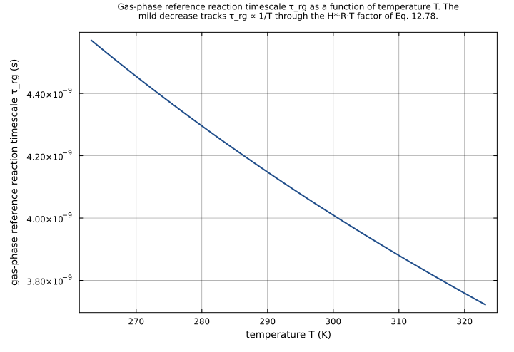
Sweep temperature from 263.15 K to 323.15 K with k_rxn and H_star at their defaults. The aqueous-phase reaction timescale τ_ra = 1/k_rxn is independent of temperature; the gas-phase reference timescale τ_rg = τ_ra/(H*·R·T) falls as 1/T because the dimensionless solubility factor H*·R·T rises with temperature.
Time span: 0.0 → 1.0
Swept over: T
rate_solubility_heatmap
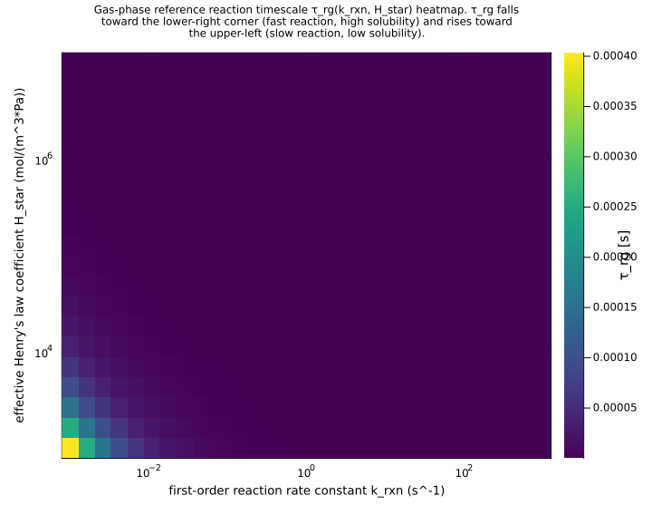
Joint dependence of the gas-phase reference reaction timescale τ_rg on the first-order reaction rate constant k_rxn and the effective Henry’s law coefficient H_star, with T at its default. τ_rg = 1/(k_rxn·H*·R·T) decreases with both a faster reaction (larger k_rxn) and a more soluble species (larger H*); the heatmap shows the product structure of Eq. 12.78.
Time span: 0.0 → 1.0
Swept over: k_rxn, H_star
Raw .esm
Raw .esm JSON (this component)
{
  "reference": {
    "citation": "Seinfeld, J. H., and Pandis, S. N. (2006). Atmospheric Chemistry and Physics: From Air Pollution to Climate Change, 2nd Edition, John Wiley & Sons, Chapter 12. Aqueous-phase reaction timescale: Eq. 12.76; gas-phase reference reaction timescale: Eq. 12.78.",
    "notes": "source_ref: Aerosol.jl@c8c640bb636b22f2425460e9ed5cba50793bfee1:src/timescales.jl:110\n\nUpstream `ReactionTimescale` is an MTK `@component` with one `@constants` entry (R, the universal gas constant), three `@parameters` (k_rxn, H_star, T), two time-indexed `@variables` (τ_ra, τ_rg), and two equations:\n  • Eq. 12.76: τ_ra ~ 1 / k_rxn — aqueous-phase reaction timescale of a first-order reaction\n  • Eq. 12.78: τ_rg ~ τ_ra / (H_star * R * T) — gas-phase reference reaction timescale\nBoth equations are algebraic (a plain `lhs ~ rhs` with no `D(·)` time derivative); the component has no differential state anywhere.\n\nObservability classification: observed-only. With no differential state, MTK `mtkcompile`/`structural_simplify` reduces the raw 2-unknown / 2-equation `System(eqs, t)` to zero ODE states plus two observed quantities recovered algebraically. τ_ra and τ_rg are therefore encoded as `type: observed`, each carrying its defining relation in its `expression` field, and the `equations` array is empty — the post-`mtkcompile` representation, matching the migration-tracker `features: ...observed` classification and sibling observed-only components critical_ssa.esm and mean_free_path.esm. τ_rg's expression references the observed variable τ_ra by name, preserving the upstream equation symbol-for-symbol; the canonical ESS runner resolves the observed-to-observed dependency, as it does in sibling tropospheric_budget.esm (observed tau_total referencing observed k_total).\n\nConstant handling: the upstream `@constants R = 8.314` migrates as a `type: parameter` with a fixed default — the ESS schema has no constant variable type, so every `@constant` becomes a fixed-default parameter (the convention sibling mean_free_path.esm applies to its R/M_air/π_val constants). `R` is one of the three reserved physical-constant names in the ESS schema (R, k_B, N_A); it is declared here with units `J/(mol*K)`, dimensionally compatible with the canonical ideal-gas-constant dimension, so it passes the schema's physical-constant unit check (parse.py `_check_physical_constant_units`).\n\nTests: the upstream component carries no test suite (migration-tracker has_tests: N). The seven inline tests below are authored directly from the two analytic formulas — τ_ra = 1/k_rxn and τ_rg = (1/k_rxn)/(H_star·R·T) — evaluated in float64 at the declared defaults or a single-parameter override. Because both outputs are algebraic and time-independent, `default_conditions` asserts at both t=0 and t=1 to confirm time-invariance; the remaining tests assert at t=0. Coverage sweeps the reaction rate constant (fast/slow first-order reaction), the effective Henry's law solubility (high/low), and the temperature (cold/warm); every test also pins τ_ra to confirm it is independent of H_star and T.\n\nTolerance rationale (model-level rel=1e-9): observed-only algebraic system, no ODE integration. τ_ra is a single division and τ_rg is a three-factor product followed by a division; float64 round-off is ~1e-15, so rel=1e-9 leaves six orders of magnitude of headroom and absorbs any associativity difference in the n-ary product H_star·R·T. The pinned expected values are the exact analytic formulas, so the migration is checkable against the textbook equations, not merely against a prior solver run.\n\nUnit balance (verified):\n  τ_ra `1 / k_rxn`: 1/(s^-1) = s\n  τ_rg `τ_ra / (H_star * R * T)`: s / (mol/(m^3*Pa) · J/(mol*K) · K) = s / (J/(m^3*Pa)); since J = Pa·m^3 the product H_star·R·T = (Pa·m^3)/(m^3·Pa) = 1 (the dimensionless effective Henry's law solubility), so τ_rg = s / 1 = s\nSI throughout; no unit conversion at parse or runtime."
  },
  "tolerance": {
    "rel": 1e-09
  },
  "variables": {
    "R": {
      "type": "parameter",
      "units": "J/(mol*K)",
      "default": 8.314,
      "description": "Universal (ideal) gas constant. Carried as a fixed-default parameter because the ESS schema has no constant variable type; the upstream value is the MTK `@constant` R = 8.314 J/(mol*K)."
    },
    "k_rxn": {
      "type": "parameter",
      "units": "s^-1",
      "default": 1.0,
      "description": "First-order rate constant of the aqueous-phase chemical reaction consuming the dissolved species. Sets the aqueous-phase reaction timescale τ_ra = 1/k_rxn."
    },
    "H_star": {
      "type": "parameter",
      "units": "mol/(m^3*Pa)",
      "default": 100000.0,
      "description": "Effective Henry's law coefficient of the species — the equilibrium ratio of dissolved (aqueous) to gas-phase abundance, enhanced where aqueous-phase dissociation or reaction increases the apparent solubility. Enters the dimensionless solubility factor H*·R·T."
    },
    "T": {
      "type": "parameter",
      "units": "K",
      "default": 298.15,
      "description": "Absolute temperature."
    },
    "τ_ra": {
      "type": "unknown",
      "units": "s",
      "description": "Aqueous-phase reaction timescale (Seinfeld & Pandis 2006, Eq. 12.76): the e-folding time τ_ra = 1/k_rxn of a dissolved species consumed by a first-order reaction of rate constant k_rxn."
    },
    "τ_rg": {
      "type": "unknown",
      "units": "s",
      "description": "Gas-phase reference reaction timescale (Seinfeld & Pandis 2006, Eq. 12.78): the aqueous-phase reaction timescale referenced to the gas phase, τ_rg = τ_ra/(H*·R·T), divided by the dimensionless effective Henry's law solubility H*·R·T. A more soluble species (larger H*) has a shorter gas-phase reference timescale."
    }
  },
  "equations": [
    {
      "lhs": "τ_ra",
      "rhs": {
        "op": "/",
        "args": [
          1.0,
          "k_rxn"
        ]
      }
    },
    {
      "lhs": "τ_rg",
      "rhs": {
        "op": "/",
        "args": [
          "τ_ra",
          {
            "op": "*",
            "args": [
              "H_star",
              "R",
              "T"
            ]
          }
        ]
      }
    }
  ],
  "tests": [
    {
      "id": "default_conditions",
      "description": "All parameters at their declared defaults: k_rxn = 1.0 s^-1, H_star = 1.0e5 mol/(m^3*Pa), T = 298.15 K, R = 8.314 J/(mol*K). The aqueous-phase reaction timescale is τ_ra = 1/k_rxn = 1.0 s. The gas-phase reference timescale is τ_rg = τ_ra/(H_star·R·T) = 1.0/(1.0e5 · 8.314 · 298.15) = 1.0/2.4788191e8 ≈ 4.0342e-9 s. Both outputs are algebraic and time-independent, so the assertions are repeated at t=0 and t=1 to confirm time-invariance.",
      "time_span": {
        "start": 0.0,
        "end": 1.0
      },
      "assertions": [
        {
          "variable": "τ_ra",
          "time": 0.0,
          "expected": 1.0
        },
        {
          "variable": "τ_rg",
          "time": 0.0,
          "expected": 4.034179016935927e-09
        },
        {
          "variable": "τ_ra",
          "time": 1.0,
          "expected": 1.0
        },
        {
          "variable": "τ_rg",
          "time": 1.0,
          "expected": 4.034179016935927e-09
        }
      ]
    },
    {
      "id": "fast_first_order_reaction",
      "description": "Fast aqueous reaction: k_rxn raised to 100.0 s^-1 (100x the default). The aqueous-phase reaction timescale shortens to τ_ra = 1/100 = 0.01 s, and the gas-phase reference timescale scales with it: τ_rg = 0.01/(1.0e5 · 8.314 · 298.15) ≈ 4.0342e-11 s. Confirms the inverse dependence τ_ra ∝ 1/k_rxn (Eq. 12.76).",
      "parameter_overrides": {
        "k_rxn": 100.0
      },
      "time_span": {
        "start": 0.0,
        "end": 1.0
      },
      "assertions": [
        {
          "variable": "τ_ra",
          "time": 0.0,
          "expected": 0.01
        },
        {
          "variable": "τ_rg",
          "time": 0.0,
          "expected": 4.034179016935928e-11
        }
      ]
    },
    {
      "id": "slow_first_order_reaction",
      "description": "Slow aqueous reaction: k_rxn lowered to 1.0e-3 s^-1 (1000x slower than the default). The aqueous-phase reaction timescale lengthens to τ_ra = 1/1.0e-3 = 1000.0 s, and the gas-phase reference timescale lengthens in proportion: τ_rg = 1000.0/(1.0e5 · 8.314 · 298.15) ≈ 4.0342e-6 s. Mirror image of `fast_first_order_reaction`.",
      "parameter_overrides": {
        "k_rxn": 0.001
      },
      "time_span": {
        "start": 0.0,
        "end": 1.0
      },
      "assertions": [
        {
          "variable": "τ_ra",
          "time": 0.0,
          "expected": 1000.0
        },
        {
          "variable": "τ_rg",
          "time": 0.0,
          "expected": 4.034179016935928e-06
        }
      ]
    },
    {
      "id": "high_effective_solubility",
      "description": "Highly soluble species: H_star raised to 1.0e7 mol/(m^3*Pa) (100x the default) with k_rxn and T at their defaults. The aqueous-phase reaction timescale τ_ra = 1/k_rxn = 1.0 s is unchanged — it does not depend on solubility — but the dimensionless solubility factor H*·R·T grows 100x, so the gas-phase reference timescale shortens to τ_rg = 1.0/(1.0e7 · 8.314 · 298.15) ≈ 4.0342e-11 s. Confirms τ_rg ∝ 1/H* (Eq. 12.78) and that τ_ra is independent of H_star.",
      "parameter_overrides": {
        "H_star": 10000000.0
      },
      "time_span": {
        "start": 0.0,
        "end": 1.0
      },
      "assertions": [
        {
          "variable": "τ_ra",
          "time": 0.0,
          "expected": 1.0
        },
        {
          "variable": "τ_rg",
          "time": 0.0,
          "expected": 4.034179016935927e-11
        }
      ]
    },
    {
      "id": "low_effective_solubility",
      "description": "Weakly soluble species: H_star lowered to 1.0e2 mol/(m^3*Pa) (1000x below the default) with k_rxn and T at their defaults. The aqueous-phase reaction timescale τ_ra = 1.0 s is again unchanged, while the gas-phase reference timescale lengthens to τ_rg = 1.0/(1.0e2 · 8.314 · 298.15) ≈ 4.0342e-6 s. Mirror image of `high_effective_solubility`.",
      "parameter_overrides": {
        "H_star": 100.0
      },
      "time_span": {
        "start": 0.0,
        "end": 1.0
      },
      "assertions": [
        {
          "variable": "τ_ra",
          "time": 0.0,
          "expected": 1.0
        },
        {
          "variable": "τ_rg",
          "time": 0.0,
          "expected": 4.034179016935928e-06
        }
      ]
    },
    {
      "id": "cold_temperature",
      "description": "Cold conditions: T lowered to 263.15 K (-10 °C, a representative supercooled-cloud temperature) with k_rxn and H_star at their defaults. The aqueous-phase reaction timescale τ_ra = 1.0 s is independent of temperature, but the dimensionless solubility factor H*·R·T falls with T, so the gas-phase reference timescale rises to τ_rg = 1.0/(1.0e5 · 8.314 · 263.15) ≈ 4.5707e-9 s. Confirms τ_rg ∝ 1/T.",
      "parameter_overrides": {
        "T": 263.15
      },
      "time_span": {
        "start": 0.0,
        "end": 1.0
      },
      "assertions": [
        {
          "variable": "τ_ra",
          "time": 0.0,
          "expected": 1.0
        },
        {
          "variable": "τ_rg",
          "time": 0.0,
          "expected": 4.5707409230455895e-09
        }
      ]
    },
    {
      "id": "warm_temperature",
      "description": "Warm conditions: T raised to 313.15 K (40 °C) with k_rxn and H_star at their defaults. The aqueous-phase reaction timescale τ_ra = 1.0 s is unchanged, while the larger H*·R·T shortens the gas-phase reference timescale to τ_rg = 1.0/(1.0e5 · 8.314 · 313.15) ≈ 3.8409e-9 s. Mirror image of `cold_temperature`.",
      "parameter_overrides": {
        "T": 313.15
      },
      "time_span": {
        "start": 0.0,
        "end": 1.0
      },
      "assertions": [
        {
          "variable": "τ_ra",
          "time": 0.0,
          "expected": 1.0
        },
        {
          "variable": "τ_rg",
          "time": 0.0,
          "expected": 3.840940360528331e-09
        }
      ]
    }
  ],
  "analyses": [
    {
      "id": "reaction_rate_sweep",
      "description": "Sweep the first-order reaction rate constant k_rxn over six orders of magnitude (1.0e-3 to 1.0e3 s^-1, logarithmically) with H_star and T at their defaults. Both timescales fall as 1/k_rxn: the aqueous-phase reaction timescale τ_ra = 1/k_rxn and the gas-phase reference timescale τ_rg = τ_ra/(H*·R·T), which is a fixed factor 1/(H*·R·T) ≈ 4.03e-9 below τ_ra at the default solubility and temperature.",
      "time_span": {
        "start": 0.0,
        "end": 1.0
      },
      "parameter_sweep": {
        "type": "cartesian",
        "dimensions": [
          {
            "parameter": "k_rxn",
            "range": {
              "start": 0.001,
              "stop": 1000.0,
              "count": 60,
              "scale": "log"
            }
          }
        ]
      },
      "plots": [
        {
          "id": "tau_ra_vs_k_rxn",
          "type": "line",
          "description": "Aqueous-phase reaction timescale τ_ra as a function of the first-order rate constant k_rxn, on log-log axes — the inverse relationship τ_ra = 1/k_rxn (Eq. 12.76).",
          "x": {
            "variable": "k_rxn",
            "label": "first-order reaction rate constant k_rxn (s^-1)"
          },
          "y": {
            "variable": "τ_ra",
            "label": "aqueous-phase reaction timescale τ_ra (s)"
          }
        },
        {
          "id": "tau_rg_vs_k_rxn",
          "type": "line",
          "description": "Gas-phase reference reaction timescale τ_rg as a function of k_rxn, on log-log axes. τ_rg ∝ 1/k_rxn, shifted below τ_ra by the dimensionless solubility factor H*·R·T (Eq. 12.78).",
          "x": {
            "variable": "k_rxn",
            "label": "first-order reaction rate constant k_rxn (s^-1)"
          },
          "y": {
            "variable": "τ_rg",
            "label": "gas-phase reference reaction timescale τ_rg (s)"
          }
        }
      ]
    },
    {
      "id": "temperature_dependence",
      "description": "Sweep temperature from 263.15 K to 323.15 K with k_rxn and H_star at their defaults. The aqueous-phase reaction timescale τ_ra = 1/k_rxn is independent of temperature; the gas-phase reference timescale τ_rg = τ_ra/(H*·R·T) falls as 1/T because the dimensionless solubility factor H*·R·T rises with temperature.",
      "time_span": {
        "start": 0.0,
        "end": 1.0
      },
      "parameter_sweep": {
        "type": "cartesian",
        "dimensions": [
          {
            "parameter": "T",
            "range": {
              "start": 263.15,
              "stop": 323.15,
              "count": 50,
              "scale": "linear"
            }
          }
        ]
      },
      "plots": [
        {
          "id": "tau_rg_vs_T",
          "type": "line",
          "description": "Gas-phase reference reaction timescale τ_rg as a function of temperature T. The mild decrease tracks τ_rg ∝ 1/T through the H*·R·T factor of Eq. 12.78.",
          "x": {
            "variable": "T",
            "label": "temperature T (K)"
          },
          "y": {
            "variable": "τ_rg",
            "label": "gas-phase reference reaction timescale τ_rg (s)"
          }
        }
      ]
    },
    {
      "id": "rate_solubility_heatmap",
      "description": "Joint dependence of the gas-phase reference reaction timescale τ_rg on the first-order reaction rate constant k_rxn and the effective Henry's law coefficient H_star, with T at its default. τ_rg = 1/(k_rxn·H*·R·T) decreases with both a faster reaction (larger k_rxn) and a more soluble species (larger H*); the heatmap shows the product structure of Eq. 12.78.",
      "time_span": {
        "start": 0.0,
        "end": 1.0
      },
      "parameter_sweep": {
        "type": "cartesian",
        "dimensions": [
          {
            "parameter": "k_rxn",
            "range": {
              "start": 0.001,
              "stop": 1000.0,
              "count": 30,
              "scale": "log"
            }
          },
          {
            "parameter": "H_star",
            "range": {
              "start": 1000.0,
              "stop": 10000000.0,
              "count": 20,
              "scale": "log"
            }
          }
        ]
      },
      "plots": [
        {
          "id": "tau_rg_heatmap",
          "type": "heatmap",
          "description": "Gas-phase reference reaction timescale τ_rg(k_rxn, H_star) heatmap. τ_rg falls toward the lower-right corner (fast reaction, high solubility) and rises toward the upper-left (slow reaction, low solubility).",
          "x": {
            "variable": "k_rxn",
            "label": "first-order reaction rate constant k_rxn (s^-1)"
          },
          "y": {
            "variable": "H_star",
            "label": "effective Henry's law coefficient H_star (mol/(m^3*Pa))"
          },
          "value": {
            "variable": "τ_rg",
            "reduce": "final"
          }
        }
      ]
    }
  ]
}