UrbanAerosol
ModelingToolkit implementation of the Urban atmospheric aerosol size distribution, from Seinfeld & Pandis (2006), Atmospheric Chemistry and Physics, 2nd ed., Chapter 8 ("Properties of the Atmospheric Aerosol"), Table 8.3. The Urban distribution is a preset of the multi-modal lognormal AerosolDistribution model: three lognormal modes (N = [99300, 1110, 36400] cm^-3, D_g = [0.013, 0.014, 0.050] um, log10 sigma = [0.245, 0.666, 0.337]) — a nucleation mode and an Aitken mode at sub-20 nm plus an accumulation mode at 50 nm, characteristic of polluted urban air. The model represents the aerosol number, surface-area and volume distributions as a sum of the three modes (Eq. 8.54) and reports the total number/surface/volume concentrations, the mode-1 Hatch-Choate diameters, and the vertical aerosol mass profile (Eq. 8.55). Migrated from Aerosol.jl UrbanAerosol, a preset wrapper around AerosolDistribution(3). Purely algebraic: ten observed outputs, no differential states, an empty equations array. The upstream length-n_modes array parameters are scalarized at n_modes = 3 with the Urban Table 8.3 mode parameters as defaults.
Description
ModelingToolkit implementation of the Urban atmospheric aerosol size distribution, from Seinfeld & Pandis (2006), Atmospheric Chemistry and Physics, 2nd ed., Chapter 8 (“Properties of the Atmospheric Aerosol”), Table 8.3. The Urban distribution is a preset of the multi-modal lognormal AerosolDistribution model: three lognormal modes (N = [99300, 1110, 36400] cm^-3, D_g = [0.013, 0.014, 0.050] um, log10 sigma = [0.245, 0.666, 0.337]) — a nucleation mode and an Aitken mode at sub-20 nm plus an accumulation mode at 50 nm, characteristic of polluted urban air. The model represents the aerosol number, surface-area and volume distributions as a sum of the three modes (Eq. 8.54) and reports the total number/surface/volume concentrations, the mode-1 Hatch-Choate diameters, and the vertical aerosol mass profile (Eq. 8.55). Migrated from Aerosol.jl UrbanAerosol, a preset wrapper around AerosolDistribution(3). Purely algebraic: ten observed outputs, no differential states, an empty equations array. The upstream length-n_modes array parameters are scalarized at n_modes = 3 with the Urban Table 8.3 mode parameters as defaults.
Reference
Seinfeld, J. H., and Pandis, S. N. (2006). Atmospheric Chemistry and Physics: From Air Pollution to Climate Change, 2nd Edition, John Wiley & Sons, Chapter 8, “Properties of the Atmospheric Aerosol”. Multi-modal lognormal size distribution: Eq. 8.54 (number), 8.49/8.50 (surface area), 8.52/8.53 (volume); Hatch-Choate diameters Eq. 8.44/8.50/8.53; total moments Eq. 8.41 with Eq. 8.5/8.7; vertical mass profile Eq. 8.55. Mode parameters are the Urban entry of Table 8.3.
_source_ref: Aerosol.jl@c8c640bb636b22f2425460e9ed5cba50793bfee1:src/size_distribution.jl:162
Upstream UrbanAerosol(; name=:UrbanAerosol) is a thin preset wrapper that calls AerosolDistribution(3; name, N_vals, D_g_vals, logsigma_vals) with the Urban mode parameters of Seinfeld & Pandis (2006) Table 8.3. It returns a flat MTK System — not a hierarchical composition — identical in structure to the base AerosolDistribution component but with the three array @parameters N / D_g / logsigma defaulted to the Urban values. The migration is therefore a standalone copy of components/aerosol/size/aerosol_distribution.esm with the nine scalarized mode-parameter defaults replaced; the ten observed-output expressions and the empty equations array are unchanged.
Migration form: observed-form, matching aerosol_distribution.esm. The base component carries two @constants (pi_c = pi, ln10 = log(10)), the length-n_modes array @parameters N / D_g / logsigma plus the scalar @parameters D_p, z, H_p, and ten time-indexed @variables (n_N_o, n_S_o, n_V_o, N_t, S_t, V_t, D_s, D_v, D_bar, M_z) each defined by one algebraic lhs ~ rhs equation whose RHS references only parameters and constants. Per the purely-algebraic migration rule each output is encoded as type: observed with its defining relation in the expression field and the equations array is empty.
Array scalarization: as in the base migration the length-3 array parameters N, D_g, logsigma are scalarized into nine scalar parameters N_1..N_3, D_g_1..D_g_3, logsigma_1..logsigma_3 and each sum(... for i in 1:n_modes) is unrolled into an explicit three-term sum. UrbanAerosol is a three-mode distribution, so n_modes = 3 is exact (not a default truncation). The .esm array-variable path emits getindex nodes (tracked upstream as gt-p3ep), which is why the scalarized form is used.
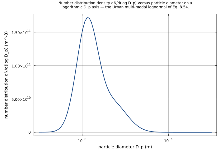
Urban defaults (Table 8.3, Seinfeld & Pandis 2006, Chapter 8): N = [99300.0, 1110.0, 36400.0] cm^-3 -> [9.93e10, 1.11e9, 3.64e10] m^-3 (x1e6); D_g = [0.013, 0.014, 0.050] um -> [1.3e-8, 1.4e-8, 5.0e-8] m (x1e-6); logsigma = [0.245, 0.666, 0.337] (log10 of the geometric standard deviation, dimensionless). Mode 1 is a nucleation mode (D_g = 0.013 um, N = 99300 cm^-3); mode 2 is an Aitken mode (D_g = 0.014 um, N = 1110 cm^-3); mode 3 is an accumulation mode (D_g = 0.050 um, N = 36400 cm^-3). Note that modes 1 and 2 have nearly identical geometric median diameters but very different widths (logsigma 0.245 vs 0.666), producing the characteristic urban bimodal nucleation+Aitken feature. D_p defaults to 1.0e-7 m (0.1 um) — the evaluation diameter used by the upstream test suite, consistent with aerosol_distribution.esm; z = 0 and H_p = 1000 m are the upstream scalar defaults.
Constant handling: pi_c and ln10 are upstream @constants. The ESS schema has no constant variable type, so each migrates as a type: parameter with a fixed evaluated numeric default (pi_c = 3.141592653589793, ln10 = 2.302585092994046); the symbols are kept in the expressions. ln10 converts the log10-based logsigma to natural-log form: ln(sigma_g) = logsigma * ln10.
Pruned parameter: the base component’s @parameter rho_p (particle density, default 1500 kg/m^3) appears in none of the ten equations and is omitted per the unused-parameter rule, as in aerosol_distribution.esm.
Tests: urban_default_distribution pins all ten outputs at the Urban defaults (D_p = 1.0e-7 m). The remaining six tests are the preset-independent equation-correctness tests carried over verbatim from aerosol_distribution.esm — they override the mode parameters (a single mode with modes 2 & 3 switched off, the lognormal one-sigma points, the near-monodisperse Hatch-Choate limit) or the vertical-profile parameters, so their expected values do not depend on the Urban defaults and verify the migrated equations directly. The Marine/Remote-continental preset-override tests of the base file are dropped — the Urban override case is reproduced here as the default-parameter test, and the other presets are off-topic.
Tolerance rationale (model-level rel=1e-9): the component is purely algebraic with no ODE integration. Each output is a finite composition of +, *, /, ^, sqrt, exp and log10 in float64 (round-off ~1e-16 relative); rel=1e-9 leaves seven orders of magnitude of headroom and absorbs any associativity difference in the n-ary sums. The urban_default_distribution expected values were generated with the canonical ESS Python runner (earthsci_ast.simulate) — the same pathway as the inline-test gate.
Units: descriptive only; the ESS runners do no dimensional analysis. Units are copied from the upstream unit metadata verbatim (n_S_o / S_t in m^-1, n_V_o / V_t / M_z dimensionless)._
Parameters
| Name | Units | Default | Description |
|---|---|---|---|
π_c | 1 | 3.141592653589793 | Pi (mathematical constant). Upstream MTK @constants entry pi_c = pi; the ESS schema has no constant variable type, so it migrates as a fixed-default parameter with the evaluated numeric value. |
ln10 | 1 | 2.302585092994046 | Natural logarithm of 10. Upstream MTK @constants entry ln10 = log(10.0); migrated as a fixed-default parameter. Converts the log10-based geometric standard deviations logsigma to natural-log form, ln(sigma_g) = logsigma * ln10. |
N_1 | m^-3 | 99300000000.0 | Total number concentration of mode 1 (nucleation mode). Upstream array @parameter N[1] of AerosolDistribution. Default: Urban distribution, Seinfeld & Pandis (2006) Table 8.3 (99300 cm^-3 converted to m^-3 by x1e6). |
N_2 | m^-3 | 1110000000.0 | Total number concentration of mode 2 (Aitken mode). Upstream array @parameter N[2] of AerosolDistribution. Default: Urban distribution, Seinfeld & Pandis (2006) Table 8.3 (1110 cm^-3 converted to m^-3 by x1e6). |
N_3 | m^-3 | 36400000000.0 | Total number concentration of mode 3 (accumulation mode). Upstream array @parameter N[3] of AerosolDistribution. Default: Urban distribution, Seinfeld & Pandis (2006) Table 8.3 (36400 cm^-3 converted to m^-3 by x1e6). |
D_g_1 | m | 1.3e-08 | Geometric median diameter of mode 1 (nucleation mode). Upstream array @parameter D_g[1] of AerosolDistribution. Default: Urban distribution, Seinfeld & Pandis (2006) Table 8.3 (0.013 um converted to m by x1e-6). |
D_g_2 | m | 1.4e-08 | Geometric median diameter of mode 2 (Aitken mode). Upstream array @parameter D_g[2] of AerosolDistribution. Default: Urban distribution, Seinfeld & Pandis (2006) Table 8.3 (0.014 um converted to m by x1e-6). |
D_g_3 | m | 5e-08 | Geometric median diameter of mode 3 (accumulation mode). Upstream array @parameter D_g[3] of AerosolDistribution. Default: Urban distribution, Seinfeld & Pandis (2006) Table 8.3 (0.050 um converted to m by x1e-6). |
logσ_1 | 1 | 0.245 | Log10 of the geometric standard deviation of mode 1 (nucleation mode) (dimensionless). Upstream array @parameter logσ[1] of AerosolDistribution. Default: Urban distribution, Seinfeld & Pandis (2006) Table 8.3. |
logσ_2 | 1 | 0.666 | Log10 of the geometric standard deviation of mode 2 (Aitken mode) (dimensionless). Upstream array @parameter logσ[2] of AerosolDistribution. Default: Urban distribution, Seinfeld & Pandis (2006) Table 8.3. |
logσ_3 | 1 | 0.337 | Log10 of the geometric standard deviation of mode 3 (accumulation mode) (dimensionless). Upstream array @parameter logσ[3] of AerosolDistribution. Default: Urban distribution, Seinfeld & Pandis (2006) Table 8.3. |
D_p | m | 1e-07 | Particle diameter at which the number, surface-area and volume distribution densities n_N_o/n_S_o/n_V_o are evaluated. The upstream base AerosolDistribution declares D_p with no default; 1.0e-7 m (0.1 um) is adopted here — the diameter the upstream test suite evaluates the distributions at, consistent with components/aerosol/size/aerosol_distribution.esm. |
z | m | 0.0 | Altitude above the surface, used by the vertical mass profile M_z. Default 0 m (surface). Upstream @parameter z = 0.0. |
H_p | m | 1000.0 | Aerosol mass scale height in the vertical profile M_z = exp(-z/H_p). Default 1000 m. Upstream @parameter H_p = 1000.0. |
Observed
| Name | Units | Default | Description |
|---|---|---|---|
n_N_o | m^-3 | Number distribution density dN/d(log D_p) at the evaluation diameter D_p — the sum of n_modes lognormal modes (Seinfeld & Pandis 2006, Eq. 8.54). | |
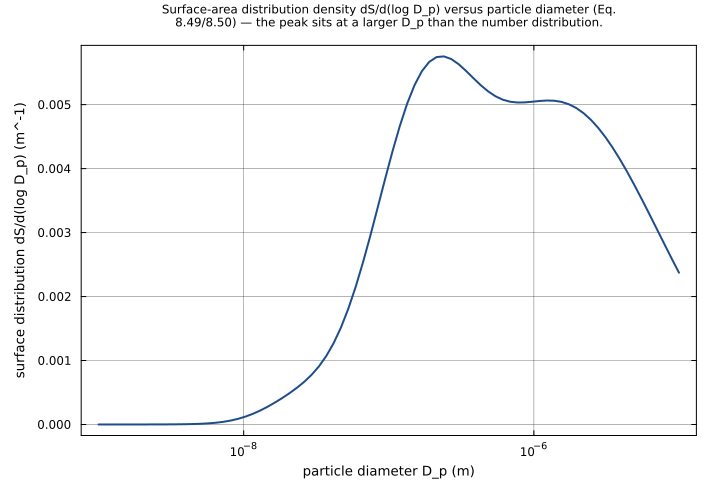
n_S_o | m^-1 | Surface-area distribution density dS/d(log D_p) at D_p (Seinfeld & Pandis 2006, Eq. 8.49/8.50). | |
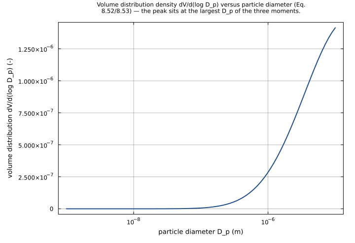
n_V_o | 1 | Volume distribution density dV/d(log D_p) at D_p (Seinfeld & Pandis 2006, Eq. 8.52/8.53). | |
N_t | m^-3 | Total number concentration — the sum of the per-mode number concentrations N_i. | |
S_t | m^-1 | Total surface-area concentration — Seinfeld & Pandis (2006) Eq. 8.5 evaluated with the k=2 lognormal moment Eq. 8.41. | |
V_t | 1 | Total volume concentration — Seinfeld & Pandis (2006) Eq. 8.7 evaluated with the k=3 lognormal moment Eq. 8.41. | |
D_s | m | Surface-area median diameter of mode 1 — the Hatch-Choate relation D_s = D_g * exp(2*ln^2 sigma_g) (Seinfeld & Pandis 2006, Eq. 8.50). | |
D_v | m | Volume median diameter of mode 1 — the Hatch-Choate relation D_v = D_g * exp(3*ln^2 sigma_g) (Seinfeld & Pandis 2006, Eq. 8.53). | |
D_bar | m | Mean diameter of mode 1 — the Hatch-Choate relation D_bar = D_g * exp(0.5*ln^2 sigma_g) (Seinfeld & Pandis 2006, Eq. 8.44). | |
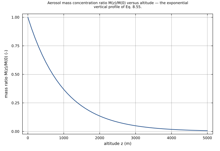
M_z | 1 | Vertical aerosol mass profile ratio M(z)/M(0) = exp(-z/H_p) (Seinfeld & Pandis 2006, Eq. 8.55), dimensionless. |
Observed expressions
$$ n_{N\,o} = \frac{N_{1}}{\sqrt{2 \cdot π_{c}} \cdot logσ_{1}} \cdot e^{\frac{-\log_{10}\left(\frac{D_{p}}{D_{g\,1}}\right)^{2}}{2 \cdot logσ_{1}^{2}}} + \frac{N_{2}}{\sqrt{2 \cdot π_{c}} \cdot logσ_{2}} \cdot e^{\frac{-\log_{10}\left(\frac{D_{p}}{D_{g\,2}}\right)^{2}}{2 \cdot logσ_{2}^{2}}} + \frac{N_{3}}{\sqrt{2 \cdot π_{c}} \cdot logσ_{3}} \cdot e^{\frac{-\log_{10}\left(\frac{D_{p}}{D_{g\,3}}\right)^{2}}{2 \cdot logσ_{3}^{2}}} $$Number distribution density dN/d(log D_p) at the evaluation diameter D_p — the sum of n_modes lognormal modes (Seinfeld & Pandis 2006, Eq. 8.54).
$$ n_{S\,o} = \frac{π_{c} \cdot N_{1} \cdot \left(D_{g\,1} \cdot e^{2 \cdot \left(logσ_{1} \cdot ln10\right)^{2}}\right)^{2}}{\sqrt{2 \cdot π_{c}} \cdot logσ_{1}} \cdot e^{\frac{-\log_{10}\left(\frac{D_{p}}{D_{g\,1} \cdot e^{2 \cdot \left(logσ_{1} \cdot ln10\right)^{2}}}\right)^{2}}{2 \cdot logσ_{1}^{2}}} + \frac{π_{c} \cdot N_{2} \cdot \left(D_{g\,2} \cdot e^{2 \cdot \left(logσ_{2} \cdot ln10\right)^{2}}\right)^{2}}{\sqrt{2 \cdot π_{c}} \cdot logσ_{2}} \cdot e^{\frac{-\log_{10}\left(\frac{D_{p}}{D_{g\,2} \cdot e^{2 \cdot \left(logσ_{2} \cdot ln10\right)^{2}}}\right)^{2}}{2 \cdot logσ_{2}^{2}}} + \frac{π_{c} \cdot N_{3} \cdot \left(D_{g\,3} \cdot e^{2 \cdot \left(logσ_{3} \cdot ln10\right)^{2}}\right)^{2}}{\sqrt{2 \cdot π_{c}} \cdot logσ_{3}} \cdot e^{\frac{-\log_{10}\left(\frac{D_{p}}{D_{g\,3} \cdot e^{2 \cdot \left(logσ_{3} \cdot ln10\right)^{2}}}\right)^{2}}{2 \cdot logσ_{3}^{2}}} $$Surface-area distribution density dS/d(log D_p) at D_p (Seinfeld & Pandis 2006, Eq. 8.49/8.50).
$$ n_{V\,o} = \frac{\frac{π_{c}}{6} \cdot N_{1} \cdot \left(D_{g\,1} \cdot e^{3 \cdot \left(logσ_{1} \cdot ln10\right)^{2}}\right)^{3}}{\sqrt{2 \cdot π_{c}} \cdot logσ_{1}} \cdot e^{\frac{-\log_{10}\left(\frac{D_{p}}{D_{g\,1} \cdot e^{3 \cdot \left(logσ_{1} \cdot ln10\right)^{2}}}\right)^{2}}{2 \cdot logσ_{1}^{2}}} + \frac{\frac{π_{c}}{6} \cdot N_{2} \cdot \left(D_{g\,2} \cdot e^{3 \cdot \left(logσ_{2} \cdot ln10\right)^{2}}\right)^{3}}{\sqrt{2 \cdot π_{c}} \cdot logσ_{2}} \cdot e^{\frac{-\log_{10}\left(\frac{D_{p}}{D_{g\,2} \cdot e^{3 \cdot \left(logσ_{2} \cdot ln10\right)^{2}}}\right)^{2}}{2 \cdot logσ_{2}^{2}}} + \frac{\frac{π_{c}}{6} \cdot N_{3} \cdot \left(D_{g\,3} \cdot e^{3 \cdot \left(logσ_{3} \cdot ln10\right)^{2}}\right)^{3}}{\sqrt{2 \cdot π_{c}} \cdot logσ_{3}} \cdot e^{\frac{-\log_{10}\left(\frac{D_{p}}{D_{g\,3} \cdot e^{3 \cdot \left(logσ_{3} \cdot ln10\right)^{2}}}\right)^{2}}{2 \cdot logσ_{3}^{2}}} $$Volume distribution density dV/d(log D_p) at D_p (Seinfeld & Pandis 2006, Eq. 8.52/8.53).
$$ N_{t} = N_{1} + N_{2} + N_{3} $$Total number concentration — the sum of the per-mode number concentrations N_i.
$$ S_{t} = π_{c} \cdot N_{1} \cdot D_{g\,1}^{2} \cdot e^{2 \cdot \left(logσ_{1} \cdot ln10\right)^{2}} + π_{c} \cdot N_{2} \cdot D_{g\,2}^{2} \cdot e^{2 \cdot \left(logσ_{2} \cdot ln10\right)^{2}} + π_{c} \cdot N_{3} \cdot D_{g\,3}^{2} \cdot e^{2 \cdot \left(logσ_{3} \cdot ln10\right)^{2}} $$Total surface-area concentration — Seinfeld & Pandis (2006) Eq. 8.5 evaluated with the k=2 lognormal moment Eq. 8.41.
$$ V_{t} = \frac{π_{c}}{6} \cdot N_{1} \cdot D_{g\,1}^{3} \cdot e^{4.5 \cdot \left(logσ_{1} \cdot ln10\right)^{2}} + \frac{π_{c}}{6} \cdot N_{2} \cdot D_{g\,2}^{3} \cdot e^{4.5 \cdot \left(logσ_{2} \cdot ln10\right)^{2}} + \frac{π_{c}}{6} \cdot N_{3} \cdot D_{g\,3}^{3} \cdot e^{4.5 \cdot \left(logσ_{3} \cdot ln10\right)^{2}} $$Total volume concentration — Seinfeld & Pandis (2006) Eq. 8.7 evaluated with the k=3 lognormal moment Eq. 8.41.
$$ D_{s} = D_{g\,1} \cdot e^{2 \cdot \left(logσ_{1} \cdot ln10\right)^{2}} $$Surface-area median diameter of mode 1 — the Hatch-Choate relation D_s = D_g * exp(2*ln^2 sigma_g) (Seinfeld & Pandis 2006, Eq. 8.50).
$$ D_{v} = D_{g\,1} \cdot e^{3 \cdot \left(logσ_{1} \cdot ln10\right)^{2}} $$Volume median diameter of mode 1 — the Hatch-Choate relation D_v = D_g * exp(3*ln^2 sigma_g) (Seinfeld & Pandis 2006, Eq. 8.53).
$$ D_{bar} = D_{g\,1} \cdot e^{0.5 \cdot \left(logσ_{1} \cdot ln10\right)^{2}} $$Mean diameter of mode 1 — the Hatch-Choate relation D_bar = D_g * exp(0.5*ln^2 sigma_g) (Seinfeld & Pandis 2006, Eq. 8.44).
$$ M_{z} = e^{-\frac{z}{H_{p}}} $$Vertical aerosol mass profile ratio M(z)/M(0) = exp(-z/H_p) (Seinfeld & Pandis 2006, Eq. 8.55), dimensionless.
Analyses
aerosol_size_distribution_curves
The Seinfeld & Pandis Chapter 8 size-distribution figure for the Urban aerosol (Table 8.3). Sweeps the evaluation diameter D_p logarithmically across the atmospheric aerosol range (1 nm to 10 um) and plots the number (n_N_o, Eq. 8.54), surface-area (n_S_o, Eq. 8.49/8.50) and volume (n_V_o, Eq. 8.52/8.53) distribution densities. The Urban distribution is dominated by nucleation and Aitken modes at very small sizes (< 20 nm); the characteristic shift of the distribution peak toward larger diameters going from number to surface to volume is the headline result.
Time span: 0.0 → 1.0
Swept over: D_p
vertical_mass_profile
Vertical aerosol mass profile of Seinfeld & Pandis Eq. 8.55. Sweeps altitude z from the surface to 5 km and plots the mass concentration ratio M_z = M(z)/M(0) = exp(-z/H_p) with the default scale height H_p = 1000 m. The profile decays exponentially, reaching 1/e of the surface value at z = H_p.
Time span: 0.0 → 1.0
Swept over: z
Raw .esm
Raw .esm JSON (this component)
{
"reference": {
"citation": "Seinfeld, J. H., and Pandis, S. N. (2006). Atmospheric Chemistry and Physics: From Air Pollution to Climate Change, 2nd Edition, John Wiley & Sons, Chapter 8, \"Properties of the Atmospheric Aerosol\". Multi-modal lognormal size distribution: Eq. 8.54 (number), 8.49/8.50 (surface area), 8.52/8.53 (volume); Hatch-Choate diameters Eq. 8.44/8.50/8.53; total moments Eq. 8.41 with Eq. 8.5/8.7; vertical mass profile Eq. 8.55. Mode parameters are the Urban entry of Table 8.3.",
"notes": "source_ref: Aerosol.jl@c8c640bb636b22f2425460e9ed5cba50793bfee1:src/size_distribution.jl:162\n\nUpstream `UrbanAerosol(; name=:UrbanAerosol)` is a thin preset wrapper that calls `AerosolDistribution(3; name, N_vals, D_g_vals, logsigma_vals)` with the Urban mode parameters of Seinfeld & Pandis (2006) Table 8.3. It returns a flat MTK `System` — not a hierarchical composition — identical in structure to the base `AerosolDistribution` component but with the three array `@parameters` N / D_g / logsigma defaulted to the Urban values. The migration is therefore a standalone copy of `components/aerosol/size/aerosol_distribution.esm` with the nine scalarized mode-parameter defaults replaced; the ten observed-output expressions and the empty equations array are unchanged.\n\nMigration form: observed-form, matching `aerosol_distribution.esm`. The base component carries two `@constants` (pi_c = pi, ln10 = log(10)), the length-n_modes array `@parameters` N / D_g / logsigma plus the scalar `@parameters` D_p, z, H_p, and ten time-indexed `@variables` (n_N_o, n_S_o, n_V_o, N_t, S_t, V_t, D_s, D_v, D_bar, M_z) each defined by one algebraic `lhs ~ rhs` equation whose RHS references only parameters and constants. Per the purely-algebraic migration rule each output is encoded as `type: observed` with its defining relation in the `expression` field and the `equations` array is empty.\n\nArray scalarization: as in the base migration the length-3 array parameters N, D_g, logsigma are scalarized into nine scalar parameters N_1..N_3, D_g_1..D_g_3, logsigma_1..logsigma_3 and each `sum(... for i in 1:n_modes)` is unrolled into an explicit three-term sum. UrbanAerosol is a three-mode distribution, so n_modes = 3 is exact (not a default truncation). The `.esm` array-variable path emits `getindex` nodes (tracked upstream as gt-p3ep), which is why the scalarized form is used.\n\nUrban defaults (Table 8.3, Seinfeld & Pandis 2006, Chapter 8): N = [99300.0, 1110.0, 36400.0] cm^-3 -> [9.93e10, 1.11e9, 3.64e10] m^-3 (x1e6); D_g = [0.013, 0.014, 0.050] um -> [1.3e-8, 1.4e-8, 5.0e-8] m (x1e-6); logsigma = [0.245, 0.666, 0.337] (log10 of the geometric standard deviation, dimensionless). Mode 1 is a nucleation mode (D_g = 0.013 um, N = 99300 cm^-3); mode 2 is an Aitken mode (D_g = 0.014 um, N = 1110 cm^-3); mode 3 is an accumulation mode (D_g = 0.050 um, N = 36400 cm^-3). Note that modes 1 and 2 have nearly identical geometric median diameters but very different widths (logsigma 0.245 vs 0.666), producing the characteristic urban bimodal nucleation+Aitken feature. D_p defaults to 1.0e-7 m (0.1 um) — the evaluation diameter used by the upstream test suite, consistent with `aerosol_distribution.esm`; z = 0 and H_p = 1000 m are the upstream scalar defaults.\n\nConstant handling: pi_c and ln10 are upstream `@constants`. The ESS schema has no constant variable type, so each migrates as a `type: parameter` with a fixed evaluated numeric default (pi_c = 3.141592653589793, ln10 = 2.302585092994046); the symbols are kept in the expressions. ln10 converts the log10-based logsigma to natural-log form: ln(sigma_g) = logsigma * ln10.\n\nPruned parameter: the base component's `@parameter rho_p` (particle density, default 1500 kg/m^3) appears in none of the ten equations and is omitted per the unused-parameter rule, as in `aerosol_distribution.esm`.\n\nTests: urban_default_distribution pins all ten outputs at the Urban defaults (D_p = 1.0e-7 m). The remaining six tests are the preset-independent equation-correctness tests carried over verbatim from `aerosol_distribution.esm` — they override the mode parameters (a single mode with modes 2 & 3 switched off, the lognormal one-sigma points, the near-monodisperse Hatch-Choate limit) or the vertical-profile parameters, so their expected values do not depend on the Urban defaults and verify the migrated equations directly. The Marine/Remote-continental preset-override tests of the base file are dropped — the Urban override case is reproduced here as the default-parameter test, and the other presets are off-topic.\n\nTolerance rationale (model-level rel=1e-9): the component is purely algebraic with no ODE integration. Each output is a finite composition of +, *, /, ^, sqrt, exp and log10 in float64 (round-off ~1e-16 relative); rel=1e-9 leaves seven orders of magnitude of headroom and absorbs any associativity difference in the n-ary sums. The urban_default_distribution expected values were generated with the canonical ESS Python runner (earthsci_ast.simulate) — the same pathway as the inline-test gate.\n\nUnits: descriptive only; the ESS runners do no dimensional analysis. Units are copied from the upstream `unit` metadata verbatim (n_S_o / S_t in m^-1, n_V_o / V_t / M_z dimensionless)."
},
"tolerance": {
"rel": 1e-09
},
"variables": {
"π_c": {
"type": "parameter",
"units": "1",
"default": 3.141592653589793,
"description": "Pi (mathematical constant). Upstream MTK @constants entry pi_c = pi; the ESS schema has no constant variable type, so it migrates as a fixed-default parameter with the evaluated numeric value."
},
"ln10": {
"type": "parameter",
"units": "1",
"default": 2.302585092994046,
"description": "Natural logarithm of 10. Upstream MTK @constants entry ln10 = log(10.0); migrated as a fixed-default parameter. Converts the log10-based geometric standard deviations logsigma to natural-log form, ln(sigma_g) = logsigma * ln10."
},
"N_1": {
"type": "parameter",
"units": "m^-3",
"default": 99300000000.0,
"description": "Total number concentration of mode 1 (nucleation mode). Upstream array @parameter N[1] of AerosolDistribution. Default: Urban distribution, Seinfeld & Pandis (2006) Table 8.3 (99300 cm^-3 converted to m^-3 by x1e6)."
},
"N_2": {
"type": "parameter",
"units": "m^-3",
"default": 1110000000.0,
"description": "Total number concentration of mode 2 (Aitken mode). Upstream array @parameter N[2] of AerosolDistribution. Default: Urban distribution, Seinfeld & Pandis (2006) Table 8.3 (1110 cm^-3 converted to m^-3 by x1e6)."
},
"N_3": {
"type": "parameter",
"units": "m^-3",
"default": 36400000000.0,
"description": "Total number concentration of mode 3 (accumulation mode). Upstream array @parameter N[3] of AerosolDistribution. Default: Urban distribution, Seinfeld & Pandis (2006) Table 8.3 (36400 cm^-3 converted to m^-3 by x1e6)."
},
"D_g_1": {
"type": "parameter",
"units": "m",
"default": 1.3e-08,
"description": "Geometric median diameter of mode 1 (nucleation mode). Upstream array @parameter D_g[1] of AerosolDistribution. Default: Urban distribution, Seinfeld & Pandis (2006) Table 8.3 (0.013 um converted to m by x1e-6)."
},
"D_g_2": {
"type": "parameter",
"units": "m",
"default": 1.4e-08,
"description": "Geometric median diameter of mode 2 (Aitken mode). Upstream array @parameter D_g[2] of AerosolDistribution. Default: Urban distribution, Seinfeld & Pandis (2006) Table 8.3 (0.014 um converted to m by x1e-6)."
},
"D_g_3": {
"type": "parameter",
"units": "m",
"default": 5e-08,
"description": "Geometric median diameter of mode 3 (accumulation mode). Upstream array @parameter D_g[3] of AerosolDistribution. Default: Urban distribution, Seinfeld & Pandis (2006) Table 8.3 (0.050 um converted to m by x1e-6)."
},
"logσ_1": {
"type": "parameter",
"units": "1",
"default": 0.245,
"description": "Log10 of the geometric standard deviation of mode 1 (nucleation mode) (dimensionless). Upstream array @parameter logσ[1] of AerosolDistribution. Default: Urban distribution, Seinfeld & Pandis (2006) Table 8.3."
},
"logσ_2": {
"type": "parameter",
"units": "1",
"default": 0.666,
"description": "Log10 of the geometric standard deviation of mode 2 (Aitken mode) (dimensionless). Upstream array @parameter logσ[2] of AerosolDistribution. Default: Urban distribution, Seinfeld & Pandis (2006) Table 8.3."
},
"logσ_3": {
"type": "parameter",
"units": "1",
"default": 0.337,
"description": "Log10 of the geometric standard deviation of mode 3 (accumulation mode) (dimensionless). Upstream array @parameter logσ[3] of AerosolDistribution. Default: Urban distribution, Seinfeld & Pandis (2006) Table 8.3."
},
"D_p": {
"type": "parameter",
"units": "m",
"default": 1e-07,
"description": "Particle diameter at which the number, surface-area and volume distribution densities n_N_o/n_S_o/n_V_o are evaluated. The upstream base AerosolDistribution declares D_p with no default; 1.0e-7 m (0.1 um) is adopted here — the diameter the upstream test suite evaluates the distributions at, consistent with components/aerosol/size/aerosol_distribution.esm."
},
"z": {
"type": "parameter",
"units": "m",
"default": 0.0,
"description": "Altitude above the surface, used by the vertical mass profile M_z. Default 0 m (surface). Upstream @parameter z = 0.0."
},
"H_p": {
"type": "parameter",
"units": "m",
"default": 1000.0,
"description": "Aerosol mass scale height in the vertical profile M_z = exp(-z/H_p). Default 1000 m. Upstream @parameter H_p = 1000.0."
},
"n_N_o": {
"type": "unknown",
"units": "m^-3",
"description": "Number distribution density dN/d(log D_p) at the evaluation diameter D_p — the sum of n_modes lognormal modes (Seinfeld & Pandis 2006, Eq. 8.54)."
},
"n_S_o": {
"type": "unknown",
"units": "m^-1",
"description": "Surface-area distribution density dS/d(log D_p) at D_p (Seinfeld & Pandis 2006, Eq. 8.49/8.50)."
},
"n_V_o": {
"type": "unknown",
"units": "1",
"description": "Volume distribution density dV/d(log D_p) at D_p (Seinfeld & Pandis 2006, Eq. 8.52/8.53)."
},
"N_t": {
"type": "unknown",
"units": "m^-3",
"description": "Total number concentration — the sum of the per-mode number concentrations N_i."
},
"S_t": {
"type": "unknown",
"units": "m^-1",
"description": "Total surface-area concentration — Seinfeld & Pandis (2006) Eq. 8.5 evaluated with the k=2 lognormal moment Eq. 8.41."
},
"V_t": {
"type": "unknown",
"units": "1",
"description": "Total volume concentration — Seinfeld & Pandis (2006) Eq. 8.7 evaluated with the k=3 lognormal moment Eq. 8.41."
},
"D_s": {
"type": "unknown",
"units": "m",
"description": "Surface-area median diameter of mode 1 — the Hatch-Choate relation D_s = D_g * exp(2*ln^2 sigma_g) (Seinfeld & Pandis 2006, Eq. 8.50)."
},
"D_v": {
"type": "unknown",
"units": "m",
"description": "Volume median diameter of mode 1 — the Hatch-Choate relation D_v = D_g * exp(3*ln^2 sigma_g) (Seinfeld & Pandis 2006, Eq. 8.53)."
},
"D_bar": {
"type": "unknown",
"units": "m",
"description": "Mean diameter of mode 1 — the Hatch-Choate relation D_bar = D_g * exp(0.5*ln^2 sigma_g) (Seinfeld & Pandis 2006, Eq. 8.44)."
},
"M_z": {
"type": "unknown",
"units": "1",
"description": "Vertical aerosol mass profile ratio M(z)/M(0) = exp(-z/H_p) (Seinfeld & Pandis 2006, Eq. 8.55), dimensionless."
}
},
"equations": [
{
"lhs": "n_N_o",
"rhs": {
"op": "+",
"args": [
{
"op": "*",
"args": [
{
"op": "/",
"args": [
"N_1",
{
"op": "*",
"args": [
{
"op": "sqrt",
"args": [
{
"op": "*",
"args": [
2,
"π_c"
]
}
]
},
"logσ_1"
]
}
]
},
{
"op": "exp",
"args": [
{
"op": "/",
"args": [
{
"op": "-",
"args": [
{
"op": "^",
"args": [
{
"op": "log10",
"args": [
{
"op": "/",
"args": [
"D_p",
"D_g_1"
]
}
]
},
2
]
}
]
},
{
"op": "*",
"args": [
2,
{
"op": "^",
"args": [
"logσ_1",
2
]
}
]
}
]
}
]
}
]
},
{
"op": "*",
"args": [
{
"op": "/",
"args": [
"N_2",
{
"op": "*",
"args": [
{
"op": "sqrt",
"args": [
{
"op": "*",
"args": [
2,
"π_c"
]
}
]
},
"logσ_2"
]
}
]
},
{
"op": "exp",
"args": [
{
"op": "/",
"args": [
{
"op": "-",
"args": [
{
"op": "^",
"args": [
{
"op": "log10",
"args": [
{
"op": "/",
"args": [
"D_p",
"D_g_2"
]
}
]
},
2
]
}
]
},
{
"op": "*",
"args": [
2,
{
"op": "^",
"args": [
"logσ_2",
2
]
}
]
}
]
}
]
}
]
},
{
"op": "*",
"args": [
{
"op": "/",
"args": [
"N_3",
{
"op": "*",
"args": [
{
"op": "sqrt",
"args": [
{
"op": "*",
"args": [
2,
"π_c"
]
}
]
},
"logσ_3"
]
}
]
},
{
"op": "exp",
"args": [
{
"op": "/",
"args": [
{
"op": "-",
"args": [
{
"op": "^",
"args": [
{
"op": "log10",
"args": [
{
"op": "/",
"args": [
"D_p",
"D_g_3"
]
}
]
},
2
]
}
]
},
{
"op": "*",
"args": [
2,
{
"op": "^",
"args": [
"logσ_3",
2
]
}
]
}
]
}
]
}
]
}
]
}
},
{
"lhs": "n_S_o",
"rhs": {
"op": "+",
"args": [
{
"op": "*",
"args": [
{
"op": "/",
"args": [
{
"op": "*",
"args": [
"π_c",
"N_1",
{
"op": "^",
"args": [
{
"op": "*",
"args": [
"D_g_1",
{
"op": "exp",
"args": [
{
"op": "*",
"args": [
2,
{
"op": "^",
"args": [
{
"op": "*",
"args": [
"logσ_1",
"ln10"
]
},
2
]
}
]
}
]
}
]
},
2
]
}
]
},
{
"op": "*",
"args": [
{
"op": "sqrt",
"args": [
{
"op": "*",
"args": [
2,
"π_c"
]
}
]
},
"logσ_1"
]
}
]
},
{
"op": "exp",
"args": [
{
"op": "/",
"args": [
{
"op": "-",
"args": [
{
"op": "^",
"args": [
{
"op": "log10",
"args": [
{
"op": "/",
"args": [
"D_p",
{
"op": "*",
"args": [
"D_g_1",
{
"op": "exp",
"args": [
{
"op": "*",
"args": [
2,
{
"op": "^",
"args": [
{
"op": "*",
"args": [
"logσ_1",
"ln10"
]
},
2
]
}
]
}
]
}
]
}
]
}
]
},
2
]
}
]
},
{
"op": "*",
"args": [
2,
{
"op": "^",
"args": [
"logσ_1",
2
]
}
]
}
]
}
]
}
]
},
{
"op": "*",
"args": [
{
"op": "/",
"args": [
{
"op": "*",
"args": [
"π_c",
"N_2",
{
"op": "^",
"args": [
{
"op": "*",
"args": [
"D_g_2",
{
"op": "exp",
"args": [
{
"op": "*",
"args": [
2,
{
"op": "^",
"args": [
{
"op": "*",
"args": [
"logσ_2",
"ln10"
]
},
2
]
}
]
}
]
}
]
},
2
]
}
]
},
{
"op": "*",
"args": [
{
"op": "sqrt",
"args": [
{
"op": "*",
"args": [
2,
"π_c"
]
}
]
},
"logσ_2"
]
}
]
},
{
"op": "exp",
"args": [
{
"op": "/",
"args": [
{
"op": "-",
"args": [
{
"op": "^",
"args": [
{
"op": "log10",
"args": [
{
"op": "/",
"args": [
"D_p",
{
"op": "*",
"args": [
"D_g_2",
{
"op": "exp",
"args": [
{
"op": "*",
"args": [
2,
{
"op": "^",
"args": [
{
"op": "*",
"args": [
"logσ_2",
"ln10"
]
},
2
]
}
]
}
]
}
]
}
]
}
]
},
2
]
}
]
},
{
"op": "*",
"args": [
2,
{
"op": "^",
"args": [
"logσ_2",
2
]
}
]
}
]
}
]
}
]
},
{
"op": "*",
"args": [
{
"op": "/",
"args": [
{
"op": "*",
"args": [
"π_c",
"N_3",
{
"op": "^",
"args": [
{
"op": "*",
"args": [
"D_g_3",
{
"op": "exp",
"args": [
{
"op": "*",
"args": [
2,
{
"op": "^",
"args": [
{
"op": "*",
"args": [
"logσ_3",
"ln10"
]
},
2
]
}
]
}
]
}
]
},
2
]
}
]
},
{
"op": "*",
"args": [
{
"op": "sqrt",
"args": [
{
"op": "*",
"args": [
2,
"π_c"
]
}
]
},
"logσ_3"
]
}
]
},
{
"op": "exp",
"args": [
{
"op": "/",
"args": [
{
"op": "-",
"args": [
{
"op": "^",
"args": [
{
"op": "log10",
"args": [
{
"op": "/",
"args": [
"D_p",
{
"op": "*",
"args": [
"D_g_3",
{
"op": "exp",
"args": [
{
"op": "*",
"args": [
2,
{
"op": "^",
"args": [
{
"op": "*",
"args": [
"logσ_3",
"ln10"
]
},
2
]
}
]
}
]
}
]
}
]
}
]
},
2
]
}
]
},
{
"op": "*",
"args": [
2,
{
"op": "^",
"args": [
"logσ_3",
2
]
}
]
}
]
}
]
}
]
}
]
}
},
{
"lhs": "n_V_o",
"rhs": {
"op": "+",
"args": [
{
"op": "*",
"args": [
{
"op": "/",
"args": [
{
"op": "*",
"args": [
{
"op": "/",
"args": [
"π_c",
6
]
},
"N_1",
{
"op": "^",
"args": [
{
"op": "*",
"args": [
"D_g_1",
{
"op": "exp",
"args": [
{
"op": "*",
"args": [
3,
{
"op": "^",
"args": [
{
"op": "*",
"args": [
"logσ_1",
"ln10"
]
},
2
]
}
]
}
]
}
]
},
3
]
}
]
},
{
"op": "*",
"args": [
{
"op": "sqrt",
"args": [
{
"op": "*",
"args": [
2,
"π_c"
]
}
]
},
"logσ_1"
]
}
]
},
{
"op": "exp",
"args": [
{
"op": "/",
"args": [
{
"op": "-",
"args": [
{
"op": "^",
"args": [
{
"op": "log10",
"args": [
{
"op": "/",
"args": [
"D_p",
{
"op": "*",
"args": [
"D_g_1",
{
"op": "exp",
"args": [
{
"op": "*",
"args": [
3,
{
"op": "^",
"args": [
{
"op": "*",
"args": [
"logσ_1",
"ln10"
]
},
2
]
}
]
}
]
}
]
}
]
}
]
},
2
]
}
]
},
{
"op": "*",
"args": [
2,
{
"op": "^",
"args": [
"logσ_1",
2
]
}
]
}
]
}
]
}
]
},
{
"op": "*",
"args": [
{
"op": "/",
"args": [
{
"op": "*",
"args": [
{
"op": "/",
"args": [
"π_c",
6
]
},
"N_2",
{
"op": "^",
"args": [
{
"op": "*",
"args": [
"D_g_2",
{
"op": "exp",
"args": [
{
"op": "*",
"args": [
3,
{
"op": "^",
"args": [
{
"op": "*",
"args": [
"logσ_2",
"ln10"
]
},
2
]
}
]
}
]
}
]
},
3
]
}
]
},
{
"op": "*",
"args": [
{
"op": "sqrt",
"args": [
{
"op": "*",
"args": [
2,
"π_c"
]
}
]
},
"logσ_2"
]
}
]
},
{
"op": "exp",
"args": [
{
"op": "/",
"args": [
{
"op": "-",
"args": [
{
"op": "^",
"args": [
{
"op": "log10",
"args": [
{
"op": "/",
"args": [
"D_p",
{
"op": "*",
"args": [
"D_g_2",
{
"op": "exp",
"args": [
{
"op": "*",
"args": [
3,
{
"op": "^",
"args": [
{
"op": "*",
"args": [
"logσ_2",
"ln10"
]
},
2
]
}
]
}
]
}
]
}
]
}
]
},
2
]
}
]
},
{
"op": "*",
"args": [
2,
{
"op": "^",
"args": [
"logσ_2",
2
]
}
]
}
]
}
]
}
]
},
{
"op": "*",
"args": [
{
"op": "/",
"args": [
{
"op": "*",
"args": [
{
"op": "/",
"args": [
"π_c",
6
]
},
"N_3",
{
"op": "^",
"args": [
{
"op": "*",
"args": [
"D_g_3",
{
"op": "exp",
"args": [
{
"op": "*",
"args": [
3,
{
"op": "^",
"args": [
{
"op": "*",
"args": [
"logσ_3",
"ln10"
]
},
2
]
}
]
}
]
}
]
},
3
]
}
]
},
{
"op": "*",
"args": [
{
"op": "sqrt",
"args": [
{
"op": "*",
"args": [
2,
"π_c"
]
}
]
},
"logσ_3"
]
}
]
},
{
"op": "exp",
"args": [
{
"op": "/",
"args": [
{
"op": "-",
"args": [
{
"op": "^",
"args": [
{
"op": "log10",
"args": [
{
"op": "/",
"args": [
"D_p",
{
"op": "*",
"args": [
"D_g_3",
{
"op": "exp",
"args": [
{
"op": "*",
"args": [
3,
{
"op": "^",
"args": [
{
"op": "*",
"args": [
"logσ_3",
"ln10"
]
},
2
]
}
]
}
]
}
]
}
]
}
]
},
2
]
}
]
},
{
"op": "*",
"args": [
2,
{
"op": "^",
"args": [
"logσ_3",
2
]
}
]
}
]
}
]
}
]
}
]
}
},
{
"lhs": "N_t",
"rhs": {
"op": "+",
"args": [
"N_1",
"N_2",
"N_3"
]
}
},
{
"lhs": "S_t",
"rhs": {
"op": "+",
"args": [
{
"op": "*",
"args": [
"π_c",
"N_1",
{
"op": "^",
"args": [
"D_g_1",
2
]
},
{
"op": "exp",
"args": [
{
"op": "*",
"args": [
2,
{
"op": "^",
"args": [
{
"op": "*",
"args": [
"logσ_1",
"ln10"
]
},
2
]
}
]
}
]
}
]
},
{
"op": "*",
"args": [
"π_c",
"N_2",
{
"op": "^",
"args": [
"D_g_2",
2
]
},
{
"op": "exp",
"args": [
{
"op": "*",
"args": [
2,
{
"op": "^",
"args": [
{
"op": "*",
"args": [
"logσ_2",
"ln10"
]
},
2
]
}
]
}
]
}
]
},
{
"op": "*",
"args": [
"π_c",
"N_3",
{
"op": "^",
"args": [
"D_g_3",
2
]
},
{
"op": "exp",
"args": [
{
"op": "*",
"args": [
2,
{
"op": "^",
"args": [
{
"op": "*",
"args": [
"logσ_3",
"ln10"
]
},
2
]
}
]
}
]
}
]
}
]
}
},
{
"lhs": "V_t",
"rhs": {
"op": "+",
"args": [
{
"op": "*",
"args": [
{
"op": "/",
"args": [
"π_c",
6
]
},
"N_1",
{
"op": "^",
"args": [
"D_g_1",
3
]
},
{
"op": "exp",
"args": [
{
"op": "*",
"args": [
4.5,
{
"op": "^",
"args": [
{
"op": "*",
"args": [
"logσ_1",
"ln10"
]
},
2
]
}
]
}
]
}
]
},
{
"op": "*",
"args": [
{
"op": "/",
"args": [
"π_c",
6
]
},
"N_2",
{
"op": "^",
"args": [
"D_g_2",
3
]
},
{
"op": "exp",
"args": [
{
"op": "*",
"args": [
4.5,
{
"op": "^",
"args": [
{
"op": "*",
"args": [
"logσ_2",
"ln10"
]
},
2
]
}
]
}
]
}
]
},
{
"op": "*",
"args": [
{
"op": "/",
"args": [
"π_c",
6
]
},
"N_3",
{
"op": "^",
"args": [
"D_g_3",
3
]
},
{
"op": "exp",
"args": [
{
"op": "*",
"args": [
4.5,
{
"op": "^",
"args": [
{
"op": "*",
"args": [
"logσ_3",
"ln10"
]
},
2
]
}
]
}
]
}
]
}
]
}
},
{
"lhs": "D_s",
"rhs": {
"op": "*",
"args": [
"D_g_1",
{
"op": "exp",
"args": [
{
"op": "*",
"args": [
2,
{
"op": "^",
"args": [
{
"op": "*",
"args": [
"logσ_1",
"ln10"
]
},
2
]
}
]
}
]
}
]
}
},
{
"lhs": "D_v",
"rhs": {
"op": "*",
"args": [
"D_g_1",
{
"op": "exp",
"args": [
{
"op": "*",
"args": [
3,
{
"op": "^",
"args": [
{
"op": "*",
"args": [
"logσ_1",
"ln10"
]
},
2
]
}
]
}
]
}
]
}
},
{
"lhs": "D_bar",
"rhs": {
"op": "*",
"args": [
"D_g_1",
{
"op": "exp",
"args": [
{
"op": "*",
"args": [
0.5,
{
"op": "^",
"args": [
{
"op": "*",
"args": [
"logσ_1",
"ln10"
]
},
2
]
}
]
}
]
}
]
}
},
{
"lhs": "M_z",
"rhs": {
"op": "exp",
"args": [
{
"op": "-",
"args": [
{
"op": "/",
"args": [
"z",
"H_p"
]
}
]
}
]
}
}
],
"tests": [
{
"id": "urban_default_distribution",
"description": "All parameters at their declared defaults — the Urban size distribution of Seinfeld & Pandis (2006) Table 8.3 (three lognormal modes: N = [99300, 1110, 36400] cm^-3, D_g = [0.013, 0.014, 0.050] um, log10 sigma = [0.245, 0.666, 0.337]; a nucleation mode and Aitken mode at sub-20 nm plus an accumulation mode at 50 nm, characteristic of polluted urban air), evaluated at D_p = 1.0e-7 m (0.1 um). Pins every one of the ten outputs: the number/surface/volume distribution densities n_N_o/n_S_o/n_V_o (Eq. 8.54/8.49/8.52), the total concentrations N_t/S_t/V_t, the mode-1 Hatch-Choate diameters D_s/D_v/D_bar, and the surface vertical mass ratio M_z. N_t = N_1+N_2+N_3 = (99300+1110+36400)e6 = 136810e9 = 1.3681e11 m^-3; M_z = exp(-z/H_p) = 1 at the surface (z = 0). All outputs are algebraic and time-independent, so N_t and M_z are also asserted at t = 1 to confirm time-invariance.",
"time_span": {
"start": 0.0,
"end": 1.0
},
"assertions": [
{
"variable": "n_N_o",
"time": 0.0,
"expected": 29440391703.87598
},
{
"variable": "n_S_o",
"time": 0.0,
"expected": 0.004055695331493581
},
{
"variable": "n_V_o",
"time": 0.0,
"expected": 6.2644540016808945e-09
},
{
"variable": "N_t",
"time": 0.0,
"expected": 136810000000.0
},
{
"variable": "S_t",
"time": 0.0,
"expected": 0.001128262200385865
},
{
"variable": "V_t",
"time": 0.0,
"expected": 9.917187382842179e-11
},
{
"variable": "D_s",
"time": 0.0,
"expected": 2.45679371670751e-08
},
{
"variable": "D_v",
"time": 0.0,
"expected": 3.377391164719613e-08
},
{
"variable": "D_bar",
"time": 0.0,
"expected": 1.524227129871013e-08
},
{
"variable": "M_z",
"time": 0.0,
"expected": 1.0
},
{
"variable": "N_t",
"time": 1.0,
"expected": 136810000000.0
},
{
"variable": "M_z",
"time": 1.0,
"expected": 1.0
}
]
},
{
"id": "single_mode_moments_and_diameters",
"description": "A single lognormal mode: N_1 = 1.0e11 m^-3, D_g_1 = 1.0e-7 m, logsigma_1 = 0.3, with modes 2 and 3 switched off (N_2 = N_3 = 0), evaluated at D_p = D_g_1 = 1.0e-7 m. This is the upstream AerosolDistribution(1) single-mode test case. At D_p = D_g the exponential in Eq. 8.54 is unity, so n_N_o reaches its peak N_1/(sqrt(2*pi)*logsigma_1). N_t = 1.0e11 m^-3. S_t and V_t reduce to the single-mode moment forms S_t = pi*N*D_g^2*exp(2*ln^2 sigma) and V_t = (pi/6)*N*D_g^3*exp(4.5*ln^2 sigma) (Eq. 8.41). The Hatch-Choate diameters satisfy D_g < D_bar < D_s < D_v (Eq. 8.44/8.50/8.53). Pins all nine.",
"parameter_overrides": {
"N_1": 100000000000.0,
"N_2": 0.0,
"N_3": 0.0,
"D_g_1": 1e-07,
"logσ_1": 0.3,
"D_p": 1e-07
},
"time_span": {
"start": 0.0,
"end": 1.0
},
"assertions": [
{
"variable": "N_t",
"time": 0.0,
"expected": 100000000000.0
},
{
"variable": "S_t",
"time": 0.0,
"expected": 0.008158591515929528
},
{
"variable": "V_t",
"time": 0.0,
"expected": 4.482761000568854e-10
},
{
"variable": "n_N_o",
"time": 0.0,
"expected": 132980760133.81091
},
{
"variable": "n_S_o",
"time": 0.0,
"expected": 0.01084935701409569
},
{
"variable": "n_V_o",
"time": 0.0,
"expected": 5.961209653538489e-10
},
{
"variable": "D_s",
"time": 0.0,
"expected": 2.596960336855569e-07
},
{
"variable": "D_v",
"time": 0.0,
"expected": 4.1850242140101953e-07
},
{
"variable": "D_bar",
"time": 0.0,
"expected": 1.2694521316234356e-07
}
]
},
{
"id": "lognormal_one_sigma_above",
"description": "Single mode (N_1 = 1.0e11, D_g_1 = 1.0e-7, logsigma_1 = 0.3, modes 2 & 3 off), evaluated one geometric standard deviation ABOVE the median diameter: D_p = D_g_1 * 10^logsigma_1. One sigma from the peak the lognormal in log-space drops by a factor exp(-0.5), so n_N_o = [N_1/(sqrt(2*pi)*logsigma_1)] * exp(-0.5) (Eq. 8.54).",
"parameter_overrides": {
"N_1": 100000000000.0,
"N_2": 0.0,
"N_3": 0.0,
"D_g_1": 1e-07,
"logσ_1": 0.3,
"D_p": 1.9952623149688795e-07
},
"time_span": {
"start": 0.0,
"end": 1.0
},
"assertions": [
{
"variable": "n_N_o",
"time": 0.0,
"expected": 80656908173.0478
}
]
},
{
"id": "lognormal_one_sigma_below",
"description": "Mirror image of lognormal_one_sigma_above: the same single mode evaluated one geometric standard deviation BELOW the median, D_p = D_g_1 * 10^-logsigma_1. The lognormal number distribution is symmetric in log(D_p) about log(D_g_1), so n_N_o here equals the one-sigma-above value to within float round-off (~13 significant figures); the pinned expected value is the exact formula output below the median, and its near-equality to lognormal_one_sigma_above verifies that log-space symmetry.",
"parameter_overrides": {
"N_1": 100000000000.0,
"N_2": 0.0,
"N_3": 0.0,
"D_g_1": 1e-07,
"logσ_1": 0.3,
"D_p": 5.011872336272722e-08
},
"time_span": {
"start": 0.0,
"end": 1.0
},
"assertions": [
{
"variable": "n_N_o",
"time": 0.0,
"expected": 80656908173.04778
}
]
},
{
"id": "vertical_profile_one_scale_height",
"description": "Vertical aerosol mass profile (Eq. 8.55), M_z = exp(-z/H_p), evaluated one scale height above the surface: z = H_p = 1000 m. M_z = exp(-1) ~ 0.3679 — the mass concentration has fallen to 1/e of its surface value.",
"parameter_overrides": {
"z": 1000.0,
"H_p": 1000.0
},
"time_span": {
"start": 0.0,
"end": 1.0
},
"assertions": [
{
"variable": "M_z",
"time": 0.0,
"expected": 0.36787944117144233
}
]
},
{
"id": "vertical_profile_two_scale_heights",
"description": "Vertical aerosol mass profile (Eq. 8.55) two scale heights up: z = 2*H_p = 2000 m with H_p = 1000 m. M_z = exp(-2) ~ 0.1353. Together with vertical_profile_one_scale_height this confirms the exponential decay M_z = exp(-z/H_p).",
"parameter_overrides": {
"z": 2000.0,
"H_p": 1000.0
},
"time_span": {
"start": 0.0,
"end": 1.0
},
"assertions": [
{
"variable": "M_z",
"time": 0.0,
"expected": 0.1353352832366127
}
]
},
{
"id": "near_monodisperse_diameters",
"description": "Near-monodisperse limit: a single mode with logsigma_1 driven to 1.0e-6 (geometric standard deviation sigma_g ~ 1). As logsigma -> 0 the Hatch-Choate corrections exp(k*ln^2 sigma) all collapse to 1, so the surface, volume and mean diameters D_s, D_v, D_bar each converge to the geometric median diameter D_g_1 = 1.0e-7 m. The pinned values are the exact formula outputs (each differs from D_g_1 by < 1.1e-11 relative). N_t = 1.0e11 m^-3.",
"parameter_overrides": {
"N_1": 100000000000.0,
"N_2": 0.0,
"N_3": 0.0,
"D_g_1": 1e-07,
"logσ_1": 1e-06,
"D_p": 1e-07
},
"time_span": {
"start": 0.0,
"end": 1.0
},
"assertions": [
{
"variable": "D_s",
"time": 0.0,
"expected": 1.0000000000106037e-07
},
{
"variable": "D_v",
"time": 0.0,
"expected": 1.0000000000159056e-07
},
{
"variable": "D_bar",
"time": 0.0,
"expected": 1.0000000000026509e-07
},
{
"variable": "N_t",
"time": 0.0,
"expected": 100000000000.0
}
]
}
],
"analyses": [
{
"id": "aerosol_size_distribution_curves",
"description": "The Seinfeld & Pandis Chapter 8 size-distribution figure for the Urban aerosol (Table 8.3). Sweeps the evaluation diameter D_p logarithmically across the atmospheric aerosol range (1 nm to 10 um) and plots the number (n_N_o, Eq. 8.54), surface-area (n_S_o, Eq. 8.49/8.50) and volume (n_V_o, Eq. 8.52/8.53) distribution densities. The Urban distribution is dominated by nucleation and Aitken modes at very small sizes (< 20 nm); the characteristic shift of the distribution peak toward larger diameters going from number to surface to volume is the headline result.",
"time_span": {
"start": 0.0,
"end": 1.0
},
"parameter_sweep": {
"type": "cartesian",
"dimensions": [
{
"parameter": "D_p",
"range": {
"start": 1e-09,
"stop": 1e-05,
"count": 80,
"scale": "log"
}
}
]
},
"plots": [
{
"id": "number_distribution",
"type": "line",
"description": "Number distribution density dN/d(log D_p) versus particle diameter on a logarithmic D_p axis — the Urban multi-modal lognormal of Eq. 8.54.",
"x": {
"variable": "D_p",
"label": "particle diameter D_p (m)"
},
"y": {
"variable": "n_N_o",
"label": "number distribution dN/d(log D_p) (m^-3)"
}
},
{
"id": "surface_distribution",
"type": "line",
"description": "Surface-area distribution density dS/d(log D_p) versus particle diameter (Eq. 8.49/8.50) — the peak sits at a larger D_p than the number distribution.",
"x": {
"variable": "D_p",
"label": "particle diameter D_p (m)"
},
"y": {
"variable": "n_S_o",
"label": "surface distribution dS/d(log D_p) (m^-1)"
}
},
{
"id": "volume_distribution",
"type": "line",
"description": "Volume distribution density dV/d(log D_p) versus particle diameter (Eq. 8.52/8.53) — the peak sits at the largest D_p of the three moments.",
"x": {
"variable": "D_p",
"label": "particle diameter D_p (m)"
},
"y": {
"variable": "n_V_o",
"label": "volume distribution dV/d(log D_p) (-)"
}
}
]
},
{
"id": "vertical_mass_profile",
"description": "Vertical aerosol mass profile of Seinfeld & Pandis Eq. 8.55. Sweeps altitude z from the surface to 5 km and plots the mass concentration ratio M_z = M(z)/M(0) = exp(-z/H_p) with the default scale height H_p = 1000 m. The profile decays exponentially, reaching 1/e of the surface value at z = H_p.",
"time_span": {
"start": 0.0,
"end": 1.0
},
"parameter_sweep": {
"type": "cartesian",
"dimensions": [
{
"parameter": "z",
"range": {
"start": 0.0,
"stop": 5000.0,
"count": 51,
"scale": "linear"
}
}
]
},
"plots": [
{
"id": "mass_ratio_vs_altitude",
"type": "line",
"description": "Aerosol mass concentration ratio M(z)/M(0) versus altitude — the exponential vertical profile of Eq. 8.55.",
"x": {
"variable": "z",
"label": "altitude z (m)"
},
"y": {
"variable": "M_z",
"label": "mass ratio M(z)/M(0) (-)"
}
}
]
}
]
}