CloudAlbedo
Cloud albedo from two-stream approximation — Seinfeld & Pandis (2006) Ch. 24 §24.8.1, Eqs. 24.37–24.38.
Description
Cloud albedo from two-stream approximation — Seinfeld & Pandis (2006) Ch. 24 §24.8.1, Eqs. 24.37–24.38.
Reference
Seinfeld, J. H., and Pandis, S. N. (2006). Atmospheric Chemistry and Physics: From Air Pollution to Climate Change, 2nd Edition, Chapter 24, Section 24.8.1, Equations 24.37–24.38.
_source_ref: Aerosol.jl@c8c640bb:src/aerosol_radiative_forcing.jl:205 Cloud albedo from two-stream approximation. Scaffolded via EarthSciAST.mtk2esm after mtkcompile, so the two algebraic equations land as observed bindings and the compiled system has zero states — the inline-test runner exercises R_c and γ at their algebraic values.
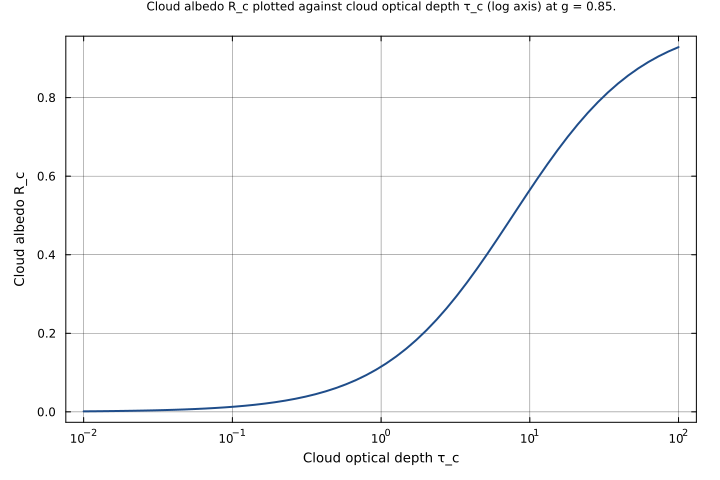
Tolerance rationale (model-level rel=1e-8 / abs=1e-12): closed-form algebraic R_c = τ_c/(τ_c+γ) reduces to zero ODE states after MTK structural_simplify, so 1e-8 captures only float64 roundoff in the (γ → R_c) two-step closed form. abs=1e-12 floors the optically-thin limit (τ_c=0.01) where R_c → ~0.001._
Parameters
| Name | Units | Default | Description |
|---|---|---|---|
τ_c | 1 | 10.0 | Cloud optical depth (dimensionless) |
g | 1 | 0.85 | Asymmetry factor (dimensionless) |
Observed
| Name | Units | Default | Description |
|---|---|---|---|
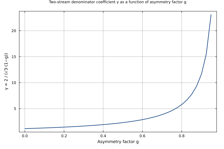
γ | 1 | Two-stream approximation denominator coefficient, γ = 2 / (√3·(1−g)). For g=0.85, γ ≈ 7.7. | |
R_c | 1 | Cloud albedo from two-stream approximation, R_c = τ_c / (τ_c + γ). |
Observed expressions
$$ γ = \frac{2}{1.7320508075688772 \cdot \left(1 + \left(-1\right) \cdot g\right)} $$Two-stream approximation denominator coefficient, γ = 2 / (√3·(1−g)). For g=0.85, γ ≈ 7.7.
$$ R_{c} = \frac{τ_{c}}{τ_{c} + γ} $$Cloud albedo from two-stream approximation, R_c = τ_c / (τ_c + γ).
Analyses
figure_24_16_r_c_vs_tau_c
Reproduces Figure 24.16 from Seinfeld & Pandis (2006), p. 1082 — cloud albedo R_c as a function of cloud optical depth τ_c at the canonical asymmetry factor g = 0.85. The curve rises from ~0 at τ_c → 0, crosses R_c = 0.5 at the diagnostic point τ_c = γ ≈ 7.7, and saturates toward 1 at large τ_c.
Time span: 0.0 → 1.0
Swept over: τ_c
asymmetry_factor_sensitivity
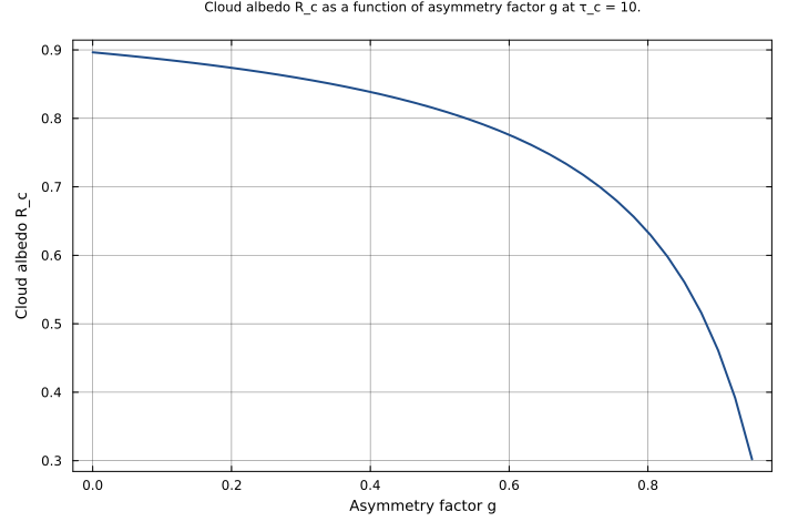
Supplements Figure 24.16 with a second sweep over the scattering asymmetry factor g (not shown in the published figure but covered by Seinfeld & Pandis §24.8.1 discussion of Eq. 24.37). At fixed τ_c = 10, increasing g from isotropic (0.0) toward strongly forward-peaked (0.95) inflates γ and suppresses R_c — the canonical justification for treating cloud droplets (g ≈ 0.85) differently from aerosols (g ≈ 0.5).
Time span: 0.0 → 1.0
Swept over: g
tau_g_joint_sweep
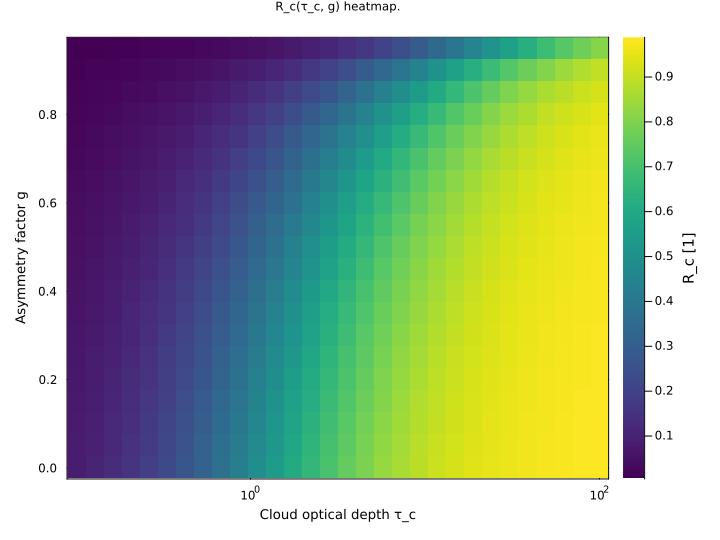
Joint sensitivity of cloud albedo to both cloud optical depth and asymmetry factor. Visualizes the Figure 24.16 curve family as a single heatmap: R_c(τ_c, g). Confirms monotonicity in both directions — R_c increases with τ_c and decreases with g.
Time span: 0.0 → 1.0
Swept over: τ_c, g
Raw .esm
Raw .esm JSON (this component)
{
  "reference": {
    "citation": "Seinfeld, J. H., and Pandis, S. N. (2006). Atmospheric Chemistry and Physics: From Air Pollution to Climate Change, 2nd Edition, Chapter 24, Section 24.8.1, Equations 24.37–24.38.",
    "notes": "source_ref: Aerosol.jl@c8c640bb:src/aerosol_radiative_forcing.jl:205\nCloud albedo from two-stream approximation. Scaffolded via EarthSciAST.mtk2esm after mtkcompile, so the two algebraic equations land as observed bindings and the compiled system has zero states — the inline-test runner exercises R_c and γ at their algebraic values.\n\nTolerance rationale (model-level rel=1e-8 / abs=1e-12): closed-form algebraic R_c = τ_c/(τ_c+γ) reduces to zero ODE states after MTK structural_simplify, so 1e-8 captures only float64 roundoff in the (γ → R_c) two-step closed form. abs=1e-12 floors the optically-thin limit (τ_c=0.01) where R_c → ~0.001."
  },
  "variables": {
    "τ_c": {
      "type": "parameter",
      "units": "1",
      "default": 10.0,
      "description": "Cloud optical depth (dimensionless)"
    },
    "g": {
      "type": "parameter",
      "units": "1",
      "default": 0.85,
      "description": "Asymmetry factor (dimensionless)"
    },
    "γ": {
      "type": "unknown",
      "units": "1",
      "description": "Two-stream approximation denominator coefficient, γ = 2 / (√3·(1−g)). For g=0.85, γ ≈ 7.7."
    },
    "R_c": {
      "type": "unknown",
      "units": "1",
      "description": "Cloud albedo from two-stream approximation, R_c = τ_c / (τ_c + γ)."
    }
  },
  "equations": [
    {
      "lhs": "γ",
      "rhs": {
        "op": "/",
        "args": [
          2,
          {
            "op": "*",
            "args": [
              1.7320508075688772,
              {
                "op": "+",
                "args": [
                  1,
                  {
                    "op": "*",
                    "args": [
                      -1,
                      "g"
                    ]
                  }
                ]
              }
            ]
          }
        ]
      }
    },
    {
      "lhs": "R_c",
      "rhs": {
        "op": "/",
        "args": [
          "τ_c",
          {
            "op": "+",
            "args": [
              "τ_c",
              "γ"
            ]
          }
        ]
      }
    }
  ],
  "tolerance": {
    "rel": 1e-08,
    "abs": 1e-12
  },
  "tests": [
    {
      "id": "figure_24_16_default_g085",
      "description": "Reproduces the γ computation and default-parameter cloud albedo from the upstream Aerosol.jl `CloudAlbedo - Figure 24.16 Validation` testitem. At g = 0.85, γ ≈ 7.698 and R_c(τ_c=10) ≈ 0.565.",
      "parameter_overrides": {
        "τ_c": 10.0,
        "g": 0.85
      },
      "time_span": {
        "start": 0.0,
        "end": 1.0
      },
      "assertions": [
        {
          "variable": "γ",
          "time": 0.0,
          "expected": 7.698003589195009
        },
        {
          "variable": "R_c",
          "time": 0.0,
          "expected": 0.5650354826521339
        },
        {
          "variable": "γ",
          "time": 1.0,
          "expected": 7.698003589195009
        },
        {
          "variable": "R_c",
          "time": 1.0,
          "expected": 0.5650354826521339
        }
      ]
    },
    {
      "id": "figure_24_16_limit_tau_near_zero",
      "description": "Optically-thin limit: τ_c ≪ γ implies R_c → 0. Upstream asserts `R_c(τ_c=0.01, g=0.85) < 0.01`; we pin the exact analytic value.",
      "parameter_overrides": {
        "τ_c": 0.01,
        "g": 0.85
      },
      "time_span": {
        "start": 0.0,
        "end": 1.0
      },
      "assertions": [
        {
          "variable": "R_c",
          "time": 0.0,
          "expected": 0.001297352794959499
        }
      ]
    },
    {
      "id": "figure_24_16_half_albedo_point",
      "description": "Half-albedo point: τ_c = γ implies R_c = 0.5 exactly. This is the canonical diagnostic marker in Figure 24.16.",
      "parameter_overrides": {
        "τ_c": 7.698003589195009,
        "g": 0.85
      },
      "time_span": {
        "start": 0.0,
        "end": 1.0
      },
      "assertions": [
        {
          "variable": "R_c",
          "time": 0.0,
          "expected": 0.5
        }
      ]
    },
    {
      "id": "figure_24_16_saturating_tau",
      "description": "Optically-thick limit: τ_c ≫ γ implies R_c → 1. Upstream asserts `R_c(τ_c=100, g=0.85) > 0.9`; we pin the analytic value.",
      "parameter_overrides": {
        "τ_c": 100.0,
        "g": 0.85
      },
      "time_span": {
        "start": 0.0,
        "end": 1.0
      },
      "assertions": [
        {
          "variable": "R_c",
          "time": 0.0,
          "expected": 0.9285223185885748
        }
      ]
    },
    {
      "id": "figure_24_16_monotonic_tau1",
      "description": "Monotonic sweep point (upstream uses τ_c ∈ {1,5,10,20,50} and asserts `issorted(R_c_vals)`). τ_c = 1.",
      "parameter_overrides": {
        "τ_c": 1.0,
        "g": 0.85
      },
      "time_span": {
        "start": 0.0,
        "end": 1.0
      },
      "assertions": [
        {
          "variable": "R_c",
          "time": 0.0,
          "expected": 0.1149689109397745
        }
      ]
    },
    {
      "id": "figure_24_16_monotonic_tau5",
      "description": "Monotonic sweep point. τ_c = 5.",
      "parameter_overrides": {
        "τ_c": 5.0,
        "g": 0.85
      },
      "time_span": {
        "start": 0.0,
        "end": 1.0
      },
      "assertions": [
        {
          "variable": "R_c",
          "time": 0.0,
          "expected": 0.3937626859906231
        }
      ]
    },
    {
      "id": "figure_24_16_monotonic_tau20",
      "description": "Monotonic sweep point. τ_c = 20.",
      "parameter_overrides": {
        "τ_c": 20.0,
        "g": 0.85
      },
      "time_span": {
        "start": 0.0,
        "end": 1.0
      },
      "assertions": [
        {
          "variable": "R_c",
          "time": 0.0,
          "expected": 0.7220737023733363
        }
      ]
    },
    {
      "id": "figure_24_16_monotonic_tau50",
      "description": "Monotonic sweep point. τ_c = 50.",
      "parameter_overrides": {
        "τ_c": 50.0,
        "g": 0.85
      },
      "time_span": {
        "start": 0.0,
        "end": 1.0
      },
      "assertions": [
        {
          "variable": "R_c",
          "time": 0.0,
          "expected": 0.866581110084776
        }
      ]
    },
    {
      "id": "asymmetry_sensitivity_low_g",
      "description": "Sensitivity to the asymmetry factor at fixed τ_c=10. g=0.5 (more isotropic scattering) yields a smaller γ and therefore a higher R_c than the g=0.85 default.",
      "parameter_overrides": {
        "τ_c": 10.0,
        "g": 0.5
      },
      "time_span": {
        "start": 0.0,
        "end": 1.0
      },
      "assertions": [
        {
          "variable": "γ",
          "time": 0.0,
          "expected": 2.309401076758503
        },
        {
          "variable": "R_c",
          "time": 0.0,
          "expected": 0.8123872102015666
        }
      ]
    },
    {
      "id": "asymmetry_sensitivity_high_g",
      "description": "Sensitivity to the asymmetry factor at fixed τ_c=10. g=0.9 (strongly forward-peaked) yields a larger γ and therefore a lower R_c than the g=0.85 default.",
      "parameter_overrides": {
        "τ_c": 10.0,
        "g": 0.9
      },
      "time_span": {
        "start": 0.0,
        "end": 1.0
      },
      "assertions": [
        {
          "variable": "γ",
          "time": 0.0,
          "expected": 11.54700538379251
        },
        {
          "variable": "R_c",
          "time": 0.0,
          "expected": 0.4641016151377546
        }
      ]
    }
  ],
  "analyses": [
    {
      "id": "figure_24_16_r_c_vs_tau_c",
      "description": "Reproduces Figure 24.16 from Seinfeld & Pandis (2006), p. 1082 — cloud albedo R_c as a function of cloud optical depth τ_c at the canonical asymmetry factor g = 0.85. The curve rises from ~0 at τ_c → 0, crosses R_c = 0.5 at the diagnostic point τ_c = γ ≈ 7.7, and saturates toward 1 at large τ_c.",
      "parameters": {
        "g": 0.85
      },
      "time_span": {
        "start": 0.0,
        "end": 1.0
      },
      "parameter_sweep": {
        "type": "cartesian",
        "dimensions": [
          {
            "parameter": "τ_c",
            "range": {
              "start": 0.01,
              "stop": 100.0,
              "count": 60,
              "scale": "log"
            }
          }
        ]
      },
      "plots": [
        {
          "id": "r_c_vs_tau_c",
          "type": "line",
          "description": "Cloud albedo R_c plotted against cloud optical depth τ_c (log axis) at g = 0.85.",
          "x": {
            "variable": "τ_c",
            "label": "Cloud optical depth τ_c"
          },
          "y": {
            "variable": "R_c",
            "label": "Cloud albedo R_c"
          }
        }
      ]
    },
    {
      "id": "asymmetry_factor_sensitivity",
      "description": "Supplements Figure 24.16 with a second sweep over the scattering asymmetry factor g (not shown in the published figure but covered by Seinfeld & Pandis §24.8.1 discussion of Eq. 24.37). At fixed τ_c = 10, increasing g from isotropic (0.0) toward strongly forward-peaked (0.95) inflates γ and suppresses R_c — the canonical justification for treating cloud droplets (g ≈ 0.85) differently from aerosols (g ≈ 0.5).",
      "parameters": {
        "τ_c": 10.0
      },
      "time_span": {
        "start": 0.0,
        "end": 1.0
      },
      "parameter_sweep": {
        "type": "cartesian",
        "dimensions": [
          {
            "parameter": "g",
            "range": {
              "start": 0.0,
              "stop": 0.95,
              "count": 40,
              "scale": "linear"
            }
          }
        ]
      },
      "plots": [
        {
          "id": "r_c_vs_g",
          "type": "line",
          "description": "Cloud albedo R_c as a function of asymmetry factor g at τ_c = 10.",
          "x": {
            "variable": "g",
            "label": "Asymmetry factor g"
          },
          "y": {
            "variable": "R_c",
            "label": "Cloud albedo R_c"
          }
        },
        {
          "id": "gamma_vs_g",
          "type": "line",
          "description": "Two-stream denominator coefficient γ as a function of asymmetry factor g.",
          "x": {
            "variable": "g",
            "label": "Asymmetry factor g"
          },
          "y": {
            "variable": "γ",
            "label": "γ = 2 / (√3·(1−g))"
          }
        }
      ]
    },
    {
      "id": "tau_g_joint_sweep",
      "description": "Joint sensitivity of cloud albedo to both cloud optical depth and asymmetry factor. Visualizes the Figure 24.16 curve family as a single heatmap: R_c(τ_c, g). Confirms monotonicity in both directions — R_c increases with τ_c and decreases with g.",
      "time_span": {
        "start": 0.0,
        "end": 1.0
      },
      "parameter_sweep": {
        "type": "cartesian",
        "dimensions": [
          {
            "parameter": "τ_c",
            "range": {
              "start": 0.1,
              "stop": 100.0,
              "count": 30,
              "scale": "log"
            }
          },
          {
            "parameter": "g",
            "range": {
              "start": 0.0,
              "stop": 0.95,
              "count": 20,
              "scale": "linear"
            }
          }
        ]
      },
      "plots": [
        {
          "id": "r_c_heatmap",
          "type": "heatmap",
          "description": "R_c(τ_c, g) heatmap.",
          "x": {
            "variable": "τ_c",
            "label": "Cloud optical depth τ_c"
          },
          "y": {
            "variable": "g",
            "label": "Asymmetry factor g"
          },
          "value": {
            "variable": "R_c",
            "reduce": "final"
          }
        }
      ]
    }
  ]
}