LangmuirAdsorption
Langmuir adsorption isotherm for the formation of a monolayer of adsorbed molecules on particle surfaces. Assumes all adsorption sites are equivalent, no horizontal interactions, and uniform heat of adsorption. From Seinfeld and Pandis (2006), Chapter 14, Section 14.5.3, Equation 14.44.
Description
Langmuir adsorption isotherm for the formation of a monolayer of adsorbed molecules on particle surfaces. Assumes all adsorption sites are equivalent, no horizontal interactions, and uniform heat of adsorption. From Seinfeld and Pandis (2006), Chapter 14, Section 14.5.3, Equation 14.44.
Reference
Seinfeld, J. H. and Pandis, S. N. (2006) Atmospheric Chemistry and Physics, 2nd Edition, Chapter 14, Section 14.5.3, Eq. 14.44 — Langmuir monolayer adsorption isotherm. Migrated from Aerosol.jl src/organic_aerosol.jl LangmuirAdsorption (esm-znc).
_source_ref: Aerosol.jl@main:src/organic_aerosol.jl:249
Upstream LangmuirAdsorption is an MTK @component with two parameters (V_m, b), and two variables (p, V). The equation is:
• V ~ V_m * b * p / (1 + b * p) (Eq. 14.44 — Langmuir isotherm)
The equation is algebraic (no derivatives), making this an observed-only component.
Observability classification: observed-only — the single output V is given by an algebraic equation in terms of input p. Test scenarios use time_span: [0, 1] and sample at t=0.
ESM representation note: in the upstream MTK component p is an @variable supplied externally as the input; in this .esm it is represented as a parameter (not a state) so the system is well-posed under the schema’s equation-count rule (one equation per state) and to match the observed-only pattern used elsewhere in this rig (see components/aerosol/organic/bet.esm). Tests vary p via parameter_overrides, and the pressure_sweep example sweeps p as a parameter dimension.
Tolerance rationale (model-level rel=1e-9): observed-only algebraic system (no ODE integration); the equation involves multiplication and division. Floating-point round-off is ~1e-15. 1e-9 leaves comfortable headroom._
Parameters
| Name | Units | Default | Description |
|---|---|---|---|
V_m | m^3 | 1.0 | Gas volume for monolayer formation |
b | Pa^-1 | 1.0 | Adsorption constant |
p | Pa | 1.0 | Gas partial pressure. Input parameter — the observed-only model has one algebraic equation for V given p. |
Observed
| Name | Units | Default | Description |
|---|---|---|---|
V | m^3 | Volume of gas adsorbed |
Observed expressions
$$ V = \frac{V_{m} \cdot b \cdot p}{1 + b \cdot p} $$Volume of gas adsorbed
Analyses
pressure_sweep
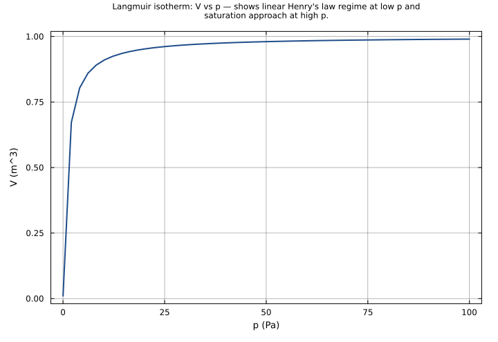
Sweep gas partial pressure from 0.01 Pa to 100 Pa to show the characteristic Langmuir isotherm shape (saturation approach as p increases).
Time span: 0.0 → 1.0
Swept over: p
Raw .esm
Raw .esm JSON (this component)
{
  "reference": {
    "citation": "Seinfeld, J. H. and Pandis, S. N. (2006) Atmospheric Chemistry and Physics, 2nd Edition, Chapter 14, Section 14.5.3, Eq. 14.44 — Langmuir monolayer adsorption isotherm. Migrated from Aerosol.jl src/organic_aerosol.jl `LangmuirAdsorption` (esm-znc).",
    "notes": "source_ref: Aerosol.jl@main:src/organic_aerosol.jl:249\nUpstream `LangmuirAdsorption` is an MTK `@component` with two parameters (V_m, b), and two variables (p, V). The equation is:\n  • V ~ V_m * b * p / (1 + b * p)  (Eq. 14.44 — Langmuir isotherm)\nThe equation is algebraic (no derivatives), making this an observed-only component.\n\nObservability classification: observed-only — the single output V is given by an algebraic equation in terms of input p. Test scenarios use `time_span: [0, 1]` and sample at t=0.\n\nESM representation note: in the upstream MTK component p is an `@variable` supplied externally as the input; in this .esm it is represented as a `parameter` (not a state) so the system is well-posed under the schema's equation-count rule (one equation per state) and to match the observed-only pattern used elsewhere in this rig (see components/aerosol/organic/bet.esm). Tests vary p via `parameter_overrides`, and the `pressure_sweep` example sweeps p as a parameter dimension.\n\nTolerance rationale (model-level rel=1e-9): observed-only algebraic system (no ODE integration); the equation involves multiplication and division. Floating-point round-off is ~1e-15. 1e-9 leaves comfortable headroom."
  },
  "tolerance": {
    "rel": 1e-09
  },
  "variables": {
    "V_m": {
      "type": "parameter",
      "units": "m^3",
      "default": 1.0,
      "description": "Gas volume for monolayer formation"
    },
    "b": {
      "type": "parameter",
      "units": "Pa^-1",
      "default": 1.0,
      "description": "Adsorption constant"
    },
    "p": {
      "type": "parameter",
      "units": "Pa",
      "default": 1.0,
      "description": "Gas partial pressure. Input parameter — the observed-only model has one algebraic equation for V given p."
    },
    "V": {
      "type": "unknown",
      "units": "m^3",
      "description": "Volume of gas adsorbed"
    }
  },
  "equations": [
    {
      "lhs": "V",
      "rhs": {
        "op": "/",
        "args": [
          {
            "op": "*",
            "args": [
              "V_m",
              "b",
              "p"
            ]
          },
          {
            "op": "+",
            "args": [
              1,
              {
                "op": "*",
                "args": [
                  "b",
                  "p"
                ]
              }
            ]
          }
        ]
      }
    }
  ],
  "tests": [
    {
      "id": "default_conditions",
      "description": "Default conditions: V_m = 1.0 m^3, b = 1.0 Pa^-1, p = 1.0 Pa. V = 1.0*1.0*1.0 / (1 + 1.0*1.0) = 1.0/2.0 = 0.5 m^3.",
      "time_span": {
        "start": 0.0,
        "end": 1.0
      },
      "parameter_overrides": {
        "p": 1.0
      },
      "assertions": [
        {
          "variable": "V",
          "time": 0.0,
          "expected": 0.5,
          "tolerance": {
            "rel": 1e-06
          }
        }
      ]
    },
    {
      "id": "high_pressure_saturation",
      "description": "High pressure: p = 1e6 Pa. V approaches V_m = 1.0 m^3 (saturation). V = 1.0*1.0*1e6 / (1 + 1.0*1e6) ≈ 0.999999.",
      "time_span": {
        "start": 0.0,
        "end": 1.0
      },
      "parameter_overrides": {
        "p": 1000000.0
      },
      "assertions": [
        {
          "variable": "V",
          "time": 0.0,
          "expected": 0.999999,
          "tolerance": {
            "rel": 0.001
          }
        }
      ]
    },
    {
      "id": "low_pressure_henry",
      "description": "Low pressure: p = 1e-6 Pa. Henry's law limit — V ≈ V_m * b * p = 1.0*1.0*1e-6 = 1e-6 m^3.",
      "time_span": {
        "start": 0.0,
        "end": 1.0
      },
      "parameter_overrides": {
        "p": 1e-06
      },
      "assertions": [
        {
          "variable": "V",
          "time": 0.0,
          "expected": 1e-06,
          "tolerance": {
            "rel": 0.001
          }
        }
      ]
    }
  ],
  "analyses": [
    {
      "id": "pressure_sweep",
      "description": "Sweep gas partial pressure from 0.01 Pa to 100 Pa to show the characteristic Langmuir isotherm shape (saturation approach as p increases).",
      "initial_state": {},
      "parameters": {
        "V_m": 1.0,
        "b": 1.0
      },
      "time_span": {
        "start": 0.0,
        "end": 1.0
      },
      "parameter_sweep": {
        "type": "cartesian",
        "dimensions": [
          {
            "parameter": "p",
            "range": {
              "start": 0.01,
              "stop": 100.0,
              "count": 50
            }
          }
        ]
      },
      "plots": [
        {
          "id": "langmuir_isotherm",
          "type": "line",
          "description": "Langmuir isotherm: V vs p — shows linear Henry's law regime at low p and saturation approach at high p.",
          "x": {
            "variable": "p",
            "label": "p (Pa)"
          },
          "y": {
            "variable": "V",
            "label": "V (m^3)"
          }
        }
      ]
    }
  ]
}