InterfaceThermalConductivity
Thermal conductivity at the interface between two adjacent thermal layers of the urban canopy column. Implements the conductivity-weighted harmonic mean (Oleson et al. 2010, CLM Tech Note Ch. 4, Eq. 4.12) derived from continuity of conductive heat flux across the interface (Eq. 4.13). Migrated from UrbanCanopy.jl@9200edd4 src/roof_wall_road_snow_temperatures.jl:278 (`InterfaceThermalConductivity` @component). Parameterized as observed-only: λ_i, λ_ip1, z_i, z_ip1, z_h are inputs (parameters); λ_interface is the algebraic output.
Description
Thermal conductivity at the interface between two adjacent thermal layers of the urban canopy column. Implements the conductivity-weighted harmonic mean (Oleson et al. 2010, CLM Tech Note Ch. 4, Eq. 4.12) derived from continuity of conductive heat flux across the interface (Eq. 4.13). Migrated from UrbanCanopy.jl@9200edd4 src/roof_wall_road_snow_temperatures.jl:278 (InterfaceThermalConductivity @component). Parameterized as observed-only: λ_i, λ_ip1, z_i, z_ip1, z_h are inputs (parameters); λ_interface is the algebraic output.
Reference
_source_ref: UrbanCanopy.jl@9200edd4f15609f20339d3a7d104de8064544310:src/roof_wall_road_snow_temperatures.jl:278
Upstream InterfaceThermalConductivity is an MTK @component whose five inputs (λ_i, λ_ip1, z_i, z_ip1, z_h) are @parameters and whose single output (λ_interface) is a time-indexed @variable with one algebraic equation (Eq. 4.12). Identical equation structure preserved here.
The upstream component declares no @constants — every input is a layer-property parameter (conductivities) or a geometry parameter (node and interface depths). The output is the conductivity-weighted harmonic mean λ[z_h] = λ_i * λ_{i+1} * (z_{i+1} - z_i) / (λ_i * (z_{i+1} - z_h) + λ_{i+1} * (z_h - z_i)) of Oleson Eq. 4.12 — derived from continuity of conductive flux at the interface (Eq. 4.13) and reducing to the simple harmonic mean 2λ_iλ_{i+1}/(λ_i + λ_{i+1}) at the midpoint z_h = (z_i + z_{i+1})/2.
Unicode parameter names (λ_i, λ_ip1, λ_interface) are preserved from upstream — the schema’s identifier pattern allows unicode and sibling observed-only ESM files in this rig already keep Greek-letter parameters from CLM nomenclature (freezing_point_depression.esm uses θ_sat, ψ_sat, ρ_liq; adjusted_layer_thickness.esm uses Δz_star). The α_CN → alpha_CN rename in heating_cooling_flux.esm was for a constant tied to that file’s HVAC algebra, not a rig-wide ban on Greek letters in identifiers.
The equation is symmetric under physical-interface coordinate flip: swapping (λ_i, z_i) ↔ (λ_{i+1}, z_{i+1}) leaves λ_interface invariant (both numerator and denominator pick up a sign flip from (z_{i+1} - z_i) and the bracketed (z_{i+1} - z_h)/(z_h - z_i) terms). This is asserted directly by the reciprocity_layer_swap test below.
Observability classification: this component is functionally observed-only — the single output variable is given by a single algebraic equation in terms of the parameters (the (t) time index has no role since there is no derivative). Test scenarios use time_span: [0, 1] and sample at t=0 to mirror the convention used by sibling observed-only ESM files in this rig (adjusted_layer_thickness.esm, freezing_point_depression.esm, total_phase_change_energy.esm, heating_cooling_flux.esm).
Tolerance rationale (model-level rel=1e-10): observed-only single-equation algebraic system (no ODE integration); the equation is two multiplications, three subtractions, one addition, and one division, so roundoff is at the IEEE-754 ULP level (~1e-16). The upstream tests use rtol = 1.0e-10 (test/roof_wall_road_snow_temperatures_test.jl:232, 243) and we mirror that for fidelity. Test assertion values are exact rationals (1.0, 1.5, 1.875, 3.0, 4.0) or short-decimal rationals (1.8, 2.4) whose IEEE-754 rounding sits below 1e-15, well within the model-level rtol._
Parameters
| Name | Units | Default | Description |
|---|---|---|---|
λ_i | W/(m*K) | 1.0 | Thermal conductivity of layer i (the upper of the two adjacent layers in the urban canopy thermal column) |
λ_ip1 | W/(m*K) | 1.0 | Thermal conductivity of layer i+1 (the lower of the two adjacent layers in the urban canopy thermal column) |
z_i | m | 0.0 | Node depth of layer i — the depth at which the layer-averaged temperature of the upper layer is carried |
z_ip1 | m | 1.0 | Node depth of layer i+1 — the depth at which the layer-averaged temperature of the lower layer is carried |
z_h | m | 0.5 | Interface depth z_{h,i} between layers i and i+1, where the interface conductivity λ_interface is evaluated (Oleson Eq. 4.12) |
Observed
| Name | Units | Default | Description |
|---|---|---|---|
λ_interface | W/(m*K) | Thermal conductivity at the interface z_h between layers i and i+1 (Oleson Eq. 4.12): λ_i * λ_ip1 * (z_ip1 - z_i) / (λ_i * (z_ip1 - z_h) + λ_ip1 * (z_h - z_i)). Reduces to the simple harmonic mean 2λ_iλ_ip1/(λ_i + λ_ip1) when z_h is the geometric midpoint. |
Observed expressions
$$ λ_{interface} = \frac{λ_{i} \cdot λ_{ip1} \cdot \left(z_{ip1} - z_{i}\right)}{λ_{i} \cdot \left(z_{ip1} - z_{h}\right) + λ_{ip1} \cdot \left(z_{h} - z_{i}\right)} $$Thermal conductivity at the interface z_h between layers i and i+1 (Oleson Eq. 4.12): λ_i * λ_ip1 * (z_ip1 - z_i) / (λ_i * (z_ip1 - z_h) + λ_ip1 * (z_h - z_i)). Reduces to the simple harmonic mean 2λ_iλ_ip1/(λ_i + λ_ip1) when z_h is the geometric midpoint.
Analyses
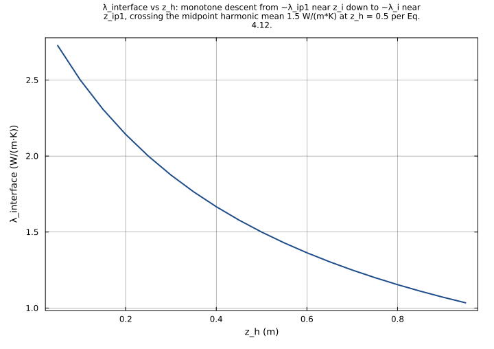
lambda_interface_vs_z_h
Sweep the interface depth z_h across the inter-node span (z_h ∈ [0.05, 0.95] m, with z_i = 0, z_ip1 = 1) at fixed conductivities λ_i = 1, λ_ip1 = 3 W/(mK). λ_interface = 131 / (1(1-z_h) + 3z_h) = 3 / (1 + 2z_h) traces a monotone decrease from λ_interface ≈ 3 (close to z_i, where the path lies almost entirely inside layer i+1 of conductivity 3) down to λ_interface ≈ 1 (close to z_ip1, where the path lies almost entirely inside layer i of conductivity 1). Crosses the midpoint harmonic mean 1.5 at z_h = 0.5 (the upstream_harmonic_mean_midpoint test value). Surfaces the geometric-weight direction of Eq. 4.12 directly.
Time span: 0.0 → 1.0
Swept over: z_h
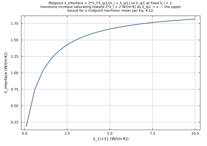
harmonic_mean_curve_vs_lambda_ip1
Sweep the lower-layer conductivity λ_ip1 ∈ [0.1, 10] W/(mK) at the midpoint interface (z_i = 0, z_ip1 = 1, z_h = 0.5) with λ_i = 1 W/(mK) fixed. λ_interface = 21λ_ip1 / (1 + λ_ip1) is the classical midpoint harmonic mean — a monotone increasing curve that approaches the asymptote 2λ_i = 2 W/(mK) as λ_ip1 → ∞ (heat flow is throttled by the lower-conductivity layer, no matter how conductive its neighbor) and crosses 1.5 W/(m*K) at λ_ip1 = 3 (matching upstream_harmonic_mean_midpoint). Surfaces the asymmetric saturation behavior central to Oleson Eq. 4.12.
Time span: 0.0 → 1.0
Swept over: λ_ip1
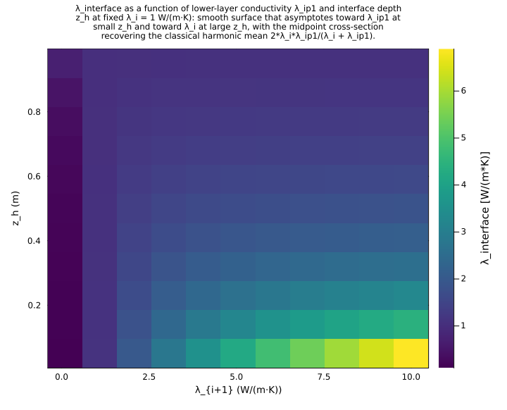
two_d_sweep_lambda_ratio_zh
Joint sweep over (λ_ip1, z_h) at fixed λ_i = 1 W/(mK) and z_i = 0, z_ip1 = 1 m. λ_interface = λ_ip1 / ((1 - z_h) + λ_ip1z_h) is a smooth surface that flattens toward λ_ip1 (=lower-layer conductivity) when z_h → 0 and toward λ_i = 1 when z_h → 1. Iso-conductivity contours show the trade-off between layer-conductivity ratio and interface position. Surfaces the full geometry-weighted harmonic-mean behavior of Eq. 4.12 across the regimes the upstream BuildingTemperature/PhaseChangeAdjustment PDE solves call this component with.
Time span: 0.0 → 1.0
Swept over: λ_ip1, z_h
Raw .esm
Raw .esm JSON (this component)
{
  "reference": {
    "notes": "source_ref: UrbanCanopy.jl@9200edd4f15609f20339d3a7d104de8064544310:src/roof_wall_road_snow_temperatures.jl:278\nUpstream `InterfaceThermalConductivity` is an MTK `@component` whose five inputs (λ_i, λ_ip1, z_i, z_ip1, z_h) are `@parameters` and whose single output (λ_interface) is a time-indexed `@variable` with one algebraic equation (Eq. 4.12). Identical equation structure preserved here.\n\nThe upstream component declares no `@constants` — every input is a layer-property parameter (conductivities) or a geometry parameter (node and interface depths). The output is the conductivity-weighted harmonic mean λ[z_h] = λ_i * λ_{i+1} * (z_{i+1} - z_i) / (λ_i * (z_{i+1} - z_h) + λ_{i+1} * (z_h - z_i)) of Oleson Eq. 4.12 — derived from continuity of conductive flux at the interface (Eq. 4.13) and reducing to the simple harmonic mean 2*λ_i*λ_{i+1}/(λ_i + λ_{i+1}) at the midpoint z_h = (z_i + z_{i+1})/2.\n\nUnicode parameter names (`λ_i`, `λ_ip1`, `λ_interface`) are preserved from upstream — the schema's identifier pattern allows unicode and sibling observed-only ESM files in this rig already keep Greek-letter parameters from CLM nomenclature (freezing_point_depression.esm uses `θ_sat`, `ψ_sat`, `ρ_liq`; adjusted_layer_thickness.esm uses `Δz_star`). The `α_CN → alpha_CN` rename in heating_cooling_flux.esm was for a constant tied to that file's HVAC algebra, not a rig-wide ban on Greek letters in identifiers.\n\nThe equation is symmetric under physical-interface coordinate flip: swapping (λ_i, z_i) ↔ (λ_{i+1}, z_{i+1}) leaves λ_interface invariant (both numerator and denominator pick up a sign flip from (z_{i+1} - z_i) and the bracketed (z_{i+1} - z_h)/(z_h - z_i) terms). This is asserted directly by the `reciprocity_layer_swap` test below.\n\nObservability classification: this component is functionally observed-only — the single output variable is given by a single algebraic equation in terms of the parameters (the `(t)` time index has no role since there is no derivative). Test scenarios use `time_span: [0, 1]` and sample at t=0 to mirror the convention used by sibling observed-only ESM files in this rig (adjusted_layer_thickness.esm, freezing_point_depression.esm, total_phase_change_energy.esm, heating_cooling_flux.esm).\n\nTolerance rationale (model-level rel=1e-10): observed-only single-equation algebraic system (no ODE integration); the equation is two multiplications, three subtractions, one addition, and one division, so roundoff is at the IEEE-754 ULP level (~1e-16). The upstream tests use `rtol = 1.0e-10` (test/roof_wall_road_snow_temperatures_test.jl:232, 243) and we mirror that for fidelity. Test assertion values are exact rationals (1.0, 1.5, 1.875, 3.0, 4.0) or short-decimal rationals (1.8, 2.4) whose IEEE-754 rounding sits below 1e-15, well within the model-level rtol."
  },
  "tolerance": {
    "rel": 1e-10
  },
  "variables": {
    "λ_i": {
      "type": "parameter",
      "units": "W/(m*K)",
      "default": 1.0,
      "description": "Thermal conductivity of layer i (the upper of the two adjacent layers in the urban canopy thermal column)"
    },
    "λ_ip1": {
      "type": "parameter",
      "units": "W/(m*K)",
      "default": 1.0,
      "description": "Thermal conductivity of layer i+1 (the lower of the two adjacent layers in the urban canopy thermal column)"
    },
    "z_i": {
      "type": "parameter",
      "units": "m",
      "default": 0.0,
      "description": "Node depth of layer i — the depth at which the layer-averaged temperature of the upper layer is carried"
    },
    "z_ip1": {
      "type": "parameter",
      "units": "m",
      "default": 1.0,
      "description": "Node depth of layer i+1 — the depth at which the layer-averaged temperature of the lower layer is carried"
    },
    "z_h": {
      "type": "parameter",
      "units": "m",
      "default": 0.5,
      "description": "Interface depth z_{h,i} between layers i and i+1, where the interface conductivity λ_interface is evaluated (Oleson Eq. 4.12)"
    },
    "λ_interface": {
      "type": "unknown",
      "units": "W/(m*K)",
      "description": "Thermal conductivity at the interface z_h between layers i and i+1 (Oleson Eq. 4.12): λ_i * λ_ip1 * (z_ip1 - z_i) / (λ_i * (z_ip1 - z_h) + λ_ip1 * (z_h - z_i)). Reduces to the simple harmonic mean 2*λ_i*λ_ip1/(λ_i + λ_ip1) when z_h is the geometric midpoint."
    }
  },
  "equations": [
    {
      "lhs": "λ_interface",
      "rhs": {
        "op": "/",
        "args": [
          {
            "op": "*",
            "args": [
              "λ_i",
              {
                "op": "*",
                "args": [
                  "λ_ip1",
                  {
                    "op": "-",
                    "args": [
                      "z_ip1",
                      "z_i"
                    ]
                  }
                ]
              }
            ]
          },
          {
            "op": "+",
            "args": [
              {
                "op": "*",
                "args": [
                  "λ_i",
                  {
                    "op": "-",
                    "args": [
                      "z_ip1",
                      "z_h"
                    ]
                  }
                ]
              },
              {
                "op": "*",
                "args": [
                  "λ_ip1",
                  {
                    "op": "-",
                    "args": [
                      "z_h",
                      "z_i"
                    ]
                  }
                ]
              }
            ]
          }
        ]
      }
    }
  ],
  "tests": [
    {
      "id": "upstream_equal_conductivities",
      "description": "Reproduces upstream `InterfaceThermalConductivity - Harmonic Mean` test case 1 (UrbanCanopy.jl test/roof_wall_road_snow_temperatures_test.jl:225-232). With equal layer conductivities (λ_i = λ_ip1 = 1.0 W/(m*K)) and a midpoint interface (z_i = 0, z_ip1 = 1, z_h = 0.5 m), Eq. 4.12 reduces to λ_interface = λ — the interface conductivity must equal the common layer value regardless of the geometric weighting in the denominator. Anchors fidelity to the upstream Julia component at this canonical fixture point.",
      "parameter_overrides": {
        "λ_i": 1.0,
        "λ_ip1": 1.0,
        "z_i": 0.0,
        "z_ip1": 1.0,
        "z_h": 0.5
      },
      "time_span": {
        "start": 0.0,
        "end": 1.0
      },
      "assertions": [
        {
          "variable": "λ_interface",
          "time": 0.0,
          "expected": 1.0
        }
      ]
    },
    {
      "id": "upstream_harmonic_mean_midpoint",
      "description": "Reproduces upstream `InterfaceThermalConductivity - Harmonic Mean` test case 2 (UrbanCanopy.jl test/roof_wall_road_snow_temperatures_test.jl:234-243). With λ_i = 1.0, λ_ip1 = 3.0 W/(m*K) and a midpoint interface (z_i = 0, z_ip1 = 1, z_h = 0.5 m), Eq. 4.12 gives λ_interface = 1*3*1 / (1*0.5 + 3*0.5) = 3/2 = 1.5 W/(m*K). At the midpoint this is exactly the harmonic mean 2*λ_i*λ_ip1/(λ_i + λ_ip1) = 6/4 = 1.5 — the upstream-test fixture used to anchor the closed-form CLM Eq. 4.12.",
      "parameter_overrides": {
        "λ_i": 1.0,
        "λ_ip1": 3.0,
        "z_i": 0.0,
        "z_ip1": 1.0,
        "z_h": 0.5
      },
      "time_span": {
        "start": 0.0,
        "end": 1.0
      },
      "assertions": [
        {
          "variable": "λ_interface",
          "time": 0.0,
          "expected": 1.5
        }
      ]
    },
    {
      "id": "midpoint_clean_ratio",
      "description": "Second independent midpoint case with a different conductivity ratio (λ_i = 2, λ_ip1 = 6 W/(m*K)) so the harmonic-mean reduction at z_h = 0.5 lands on a different rational: λ_interface = 2*6*1 / (2*0.5 + 6*0.5) = 12/4 = 3.0 W/(m*K). Confirms the equation handles non-(1, 3) conductivity pairs correctly and pins a second exact reference point for the midpoint harmonic-mean branch.",
      "parameter_overrides": {
        "λ_i": 2.0,
        "λ_ip1": 6.0,
        "z_i": 0.0,
        "z_ip1": 1.0,
        "z_h": 0.5
      },
      "time_span": {
        "start": 0.0,
        "end": 1.0
      },
      "assertions": [
        {
          "variable": "λ_interface",
          "time": 0.0,
          "expected": 3.0
        }
      ]
    },
    {
      "id": "interface_off_center_toward_layer_i",
      "description": "Off-center interface placed closer to layer i's node (z_h = 0.25, with z_i = 0, z_ip1 = 1): more of the inter-node path lies inside layer i+1, so the harmonic mean leans toward λ_ip1. With λ_i = 2, λ_ip1 = 6 W/(m*K), Eq. 4.12 gives λ_interface = 2*6*1 / (2*0.75 + 6*0.25) = 12/(1.5 + 1.5) = 12/3 = 4.0 W/(m*K). Compared with the 3.0 W/(m*K) midpoint value (`midpoint_clean_ratio`), the shift toward 4.0 — closer to λ_ip1 = 6 than to λ_i = 2 — confirms the upstream geometry-weighted direction of Eq. 4.12.",
      "parameter_overrides": {
        "λ_i": 2.0,
        "λ_ip1": 6.0,
        "z_i": 0.0,
        "z_ip1": 1.0,
        "z_h": 0.25
      },
      "time_span": {
        "start": 0.0,
        "end": 1.0
      },
      "assertions": [
        {
          "variable": "λ_interface",
          "time": 0.0,
          "expected": 4.0
        }
      ]
    },
    {
      "id": "interface_off_center_toward_layer_ip1",
      "description": "Off-center interface placed closer to layer i+1's node (z_h = 0.75, with z_i = 0, z_ip1 = 1): more of the inter-node path lies inside layer i, so the harmonic mean leans toward λ_i. With λ_i = 2, λ_ip1 = 6 W/(m*K), Eq. 4.12 gives λ_interface = 2*6*1 / (2*0.25 + 6*0.75) = 12/(0.5 + 4.5) = 12/5 = 2.4 W/(m*K). Compared with the 3.0 W/(m*K) midpoint value, the shift toward 2.4 — closer to λ_i = 2 than to λ_ip1 = 6 — confirms the upstream geometry-weighted direction. Pairs with `interface_off_center_toward_layer_i` to bracket the z_h sensitivity symmetrically around the midpoint.",
      "parameter_overrides": {
        "λ_i": 2.0,
        "λ_ip1": 6.0,
        "z_i": 0.0,
        "z_ip1": 1.0,
        "z_h": 0.75
      },
      "time_span": {
        "start": 0.0,
        "end": 1.0
      },
      "assertions": [
        {
          "variable": "λ_interface",
          "time": 0.0,
          "expected": 2.4
        }
      ]
    },
    {
      "id": "equal_conductivities_off_center_z_h",
      "description": "Equal layer conductivities (λ_i = λ_ip1 = 1.5 W/(m*K)) with an off-center interface (z_h = 0.3, with z_i = 0, z_ip1 = 1): Eq. 4.12 still collapses to the common λ value because the numerator factors λ*λ*(z_ip1 - z_i) and the denominator factors λ*((z_ip1 - z_h) + (z_h - z_i)) = λ*(z_ip1 - z_i), so the geometric weighting cancels identically. Confirms the equation correctly identifies the trivial limit at any z_h ∈ (z_i, z_ip1) — pairs with `upstream_equal_conductivities` to verify z_h-independence in the equal-λ regime.",
      "parameter_overrides": {
        "λ_i": 1.5,
        "λ_ip1": 1.5,
        "z_i": 0.0,
        "z_ip1": 1.0,
        "z_h": 0.3
      },
      "time_span": {
        "start": 0.0,
        "end": 1.0
      },
      "assertions": [
        {
          "variable": "λ_interface",
          "time": 0.0,
          "expected": 1.5
        }
      ]
    },
    {
      "id": "insulator_over_conductor_thin_layer",
      "description": "Large conductivity contrast representative of an insulating top layer over a conducting subsurface — e.g., a low-conductivity roofing material over a structural sublayer (λ_i = 1, λ_ip1 = 9 W/(m*K), ratio 1:9) with a thin sub-decimetre layer (z_i = 0, z_ip1 = 0.1 m, z_h = 0.05 m at midpoint). Eq. 4.12 gives λ_interface = 1*9*0.1 / (1*0.05 + 9*0.05) = 0.9/0.5 = 1.8 W/(m*K). This is the standard midpoint harmonic mean 2*λ_i*λ_ip1/(λ_i + λ_ip1) = 18/10 = 1.8 — the result is dominated by the lower-conductivity layer (closer to λ_i = 1 than to λ_ip1 = 9) as expected from the harmonic-mean limit. Exercises the equation in the large-contrast regime that drives urban roof/wall heat-flux discretization.",
      "parameter_overrides": {
        "λ_i": 1.0,
        "λ_ip1": 9.0,
        "z_i": 0.0,
        "z_ip1": 0.1,
        "z_h": 0.05
      },
      "time_span": {
        "start": 0.0,
        "end": 1.0
      },
      "assertions": [
        {
          "variable": "λ_interface",
          "time": 0.0,
          "expected": 1.8
        }
      ]
    },
    {
      "id": "reciprocity_layer_swap",
      "description": "Reciprocity / coordinate-flip symmetry: viewing the same physical interface from the opposite direction must give the same λ_interface. Setup mirrors `upstream_harmonic_mean_midpoint` (λ_i = 1, λ_ip1 = 3, z_i = 0, z_ip1 = 1, z_h = 0.5 → 1.5) but with the labels swapped (λ_i = 3, λ_ip1 = 1, z_i = 1, z_ip1 = 0, z_h = 0.5). Eq. 4.12 gives λ_interface = 3*1*(0-1) / (3*(0-0.5) + 1*(0.5-1)) = -3/(-1.5 - 0.5) = -3/-2 = 1.5 W/(m*K) — sign flips in both numerator and denominator cancel. Verifies the equation does not encode any directional preference for which side of the interface is labeled `i`.",
      "parameter_overrides": {
        "λ_i": 3.0,
        "λ_ip1": 1.0,
        "z_i": 1.0,
        "z_ip1": 0.0,
        "z_h": 0.5
      },
      "time_span": {
        "start": 0.0,
        "end": 1.0
      },
      "assertions": [
        {
          "variable": "λ_interface",
          "time": 0.0,
          "expected": 1.5
        }
      ]
    },
    {
      "id": "deep_subgrade_dense_soil_over_bedrock",
      "description": "Realistic mid-column CLM road geometry with a soil layer above a denser, more conductive bedrock-like sublayer: λ_i = 1.5 W/(m*K) (typical wet soil), λ_ip1 = 2.5 W/(m*K) (consolidated saprolite/bedrock), z_i = 0.5 m, z_ip1 = 1.5 m, z_h = 1.0 m (midpoint). Eq. 4.12 gives λ_interface = 1.5*2.5*1.0 / (1.5*0.5 + 2.5*0.5) = 3.75/2.0 = 1.875 W/(m*K). Exercises the equation in the mid-column physical regime targeted by Oleson Sec. 4.1 (away from the surface-layer fixtures used in the upstream tests) with non-zero z_i.",
      "parameter_overrides": {
        "λ_i": 1.5,
        "λ_ip1": 2.5,
        "z_i": 0.5,
        "z_ip1": 1.5,
        "z_h": 1.0
      },
      "time_span": {
        "start": 0.0,
        "end": 1.0
      },
      "assertions": [
        {
          "variable": "λ_interface",
          "time": 0.0,
          "expected": 1.875
        }
      ]
    }
  ],
  "analyses": [
    {
      "id": "lambda_interface_vs_z_h",
      "description": "Sweep the interface depth z_h across the inter-node span (z_h ∈ [0.05, 0.95] m, with z_i = 0, z_ip1 = 1) at fixed conductivities λ_i = 1, λ_ip1 = 3 W/(m*K). λ_interface = 1*3*1 / (1*(1-z_h) + 3*z_h) = 3 / (1 + 2*z_h) traces a monotone decrease from λ_interface ≈ 3 (close to z_i, where the path lies almost entirely inside layer i+1 of conductivity 3) down to λ_interface ≈ 1 (close to z_ip1, where the path lies almost entirely inside layer i of conductivity 1). Crosses the midpoint harmonic mean 1.5 at z_h = 0.5 (the `upstream_harmonic_mean_midpoint` test value). Surfaces the geometric-weight direction of Eq. 4.12 directly.",
      "initial_state": {},
      "parameters": {
        "λ_i": 1.0,
        "λ_ip1": 3.0,
        "z_i": 0.0,
        "z_ip1": 1.0
      },
      "time_span": {
        "start": 0.0,
        "end": 1.0
      },
      "parameter_sweep": {
        "type": "cartesian",
        "dimensions": [
          {
            "parameter": "z_h",
            "range": {
              "start": 0.05,
              "stop": 0.95,
              "count": 19,
              "scale": "linear"
            }
          }
        ]
      },
      "plots": [
        {
          "id": "lambda_interface_curve",
          "type": "line",
          "description": "λ_interface vs z_h: monotone descent from ~λ_ip1 near z_i down to ~λ_i near z_ip1, crossing the midpoint harmonic mean 1.5 W/(m*K) at z_h = 0.5 per Eq. 4.12.",
          "x": {
            "variable": "z_h",
            "label": "z_h (m)"
          },
          "y": {
            "variable": "λ_interface",
            "label": "λ_interface (W/(m·K))"
          }
        }
      ]
    },
    {
      "id": "harmonic_mean_curve_vs_lambda_ip1",
      "description": "Sweep the lower-layer conductivity λ_ip1 ∈ [0.1, 10] W/(m*K) at the midpoint interface (z_i = 0, z_ip1 = 1, z_h = 0.5) with λ_i = 1 W/(m*K) fixed. λ_interface = 2*1*λ_ip1 / (1 + λ_ip1) is the classical midpoint harmonic mean — a monotone increasing curve that approaches the asymptote 2*λ_i = 2 W/(m*K) as λ_ip1 → ∞ (heat flow is throttled by the lower-conductivity layer, no matter how conductive its neighbor) and crosses 1.5 W/(m*K) at λ_ip1 = 3 (matching `upstream_harmonic_mean_midpoint`). Surfaces the asymmetric saturation behavior central to Oleson Eq. 4.12.",
      "initial_state": {},
      "parameters": {
        "λ_i": 1.0,
        "z_i": 0.0,
        "z_ip1": 1.0,
        "z_h": 0.5
      },
      "time_span": {
        "start": 0.0,
        "end": 1.0
      },
      "parameter_sweep": {
        "type": "cartesian",
        "dimensions": [
          {
            "parameter": "λ_ip1",
            "range": {
              "start": 0.1,
              "stop": 10.0,
              "count": 21,
              "scale": "linear"
            }
          }
        ]
      },
      "plots": [
        {
          "id": "harmonic_mean_curve",
          "type": "line",
          "description": "Midpoint λ_interface = 2*λ_i*λ_ip1/(λ_i + λ_ip1) vs λ_ip1 at fixed λ_i = 1: monotone increase saturating toward 2*λ_i = 2 W/(m·K) as λ_ip1 → ∞ — the upper bound for a midpoint harmonic mean per Eq. 4.12.",
          "x": {
            "variable": "λ_ip1",
            "label": "λ_{i+1} (W/(m·K))"
          },
          "y": {
            "variable": "λ_interface",
            "label": "λ_interface (W/(m·K))"
          }
        }
      ]
    },
    {
      "id": "two_d_sweep_lambda_ratio_zh",
      "description": "Joint sweep over (λ_ip1, z_h) at fixed λ_i = 1 W/(m*K) and z_i = 0, z_ip1 = 1 m. λ_interface = λ_ip1 / ((1 - z_h) + λ_ip1*z_h) is a smooth surface that flattens toward λ_ip1 (=lower-layer conductivity) when z_h → 0 and toward λ_i = 1 when z_h → 1. Iso-conductivity contours show the trade-off between layer-conductivity ratio and interface position. Surfaces the full geometry-weighted harmonic-mean behavior of Eq. 4.12 across the regimes the upstream `BuildingTemperature`/`PhaseChangeAdjustment` PDE solves call this component with.",
      "initial_state": {},
      "parameters": {
        "λ_i": 1.0,
        "z_i": 0.0,
        "z_ip1": 1.0
      },
      "time_span": {
        "start": 0.0,
        "end": 1.0
      },
      "parameter_sweep": {
        "type": "cartesian",
        "dimensions": [
          {
            "parameter": "λ_ip1",
            "range": {
              "start": 0.1,
              "stop": 10.0,
              "count": 11,
              "scale": "linear"
            }
          },
          {
            "parameter": "z_h",
            "range": {
              "start": 0.05,
              "stop": 0.95,
              "count": 11,
              "scale": "linear"
            }
          }
        ]
      },
      "plots": [
        {
          "id": "lambda_interface_heatmap",
          "type": "heatmap",
          "description": "λ_interface as a function of lower-layer conductivity λ_ip1 and interface depth z_h at fixed λ_i = 1 W/(m·K): smooth surface that asymptotes toward λ_ip1 at small z_h and toward λ_i at large z_h, with the midpoint cross-section recovering the classical harmonic mean 2*λ_i*λ_ip1/(λ_i + λ_ip1).",
          "x": {
            "variable": "λ_ip1",
            "label": "λ_{i+1} (W/(m·K))"
          },
          "y": {
            "variable": "z_h",
            "label": "z_h (m)"
          },
          "value": {
            "variable": "λ_interface",
            "reduce": "final"
          }
        }
      ]
    }
  ]
}