SoilWaterFlux
Soil water flux at the interface between two adjacent soil layers, computed from Darcy's law with the Zeng and Decker (2009) equilibrium-potential correction (Oleson et al. 2010, CLM4 Tech Note Eq. 5.88). q = -k_interface * ((ψ_upper - ψ_lower) + (ψ_E_lower - ψ_E_upper)) / (z_lower - z_upper), positive upward. Migrated from UrbanCanopy.jl@9200edd4 src/hydrology.jl:471 (`SoilWaterFlux` @component). Observed-only: the seven inputs are parameters and q is given by a single algebraic equation.
Description
Soil water flux at the interface between two adjacent soil layers, computed from Darcy’s law with the Zeng and Decker (2009) equilibrium-potential correction (Oleson et al. 2010, CLM4 Tech Note Eq. 5.88). q = -k_interface * ((ψ_upper - ψ_lower) + (ψ_E_lower - ψ_E_upper)) / (z_lower - z_upper), positive upward. Migrated from UrbanCanopy.jl@9200edd4 src/hydrology.jl:471 (SoilWaterFlux @component). Observed-only: the seven inputs are parameters and q is given by a single algebraic equation.
Reference
_source_ref: UrbanCanopy.jl@9200edd4f15609f20339d3a7d104de8064544310:src/hydrology.jl:471
Upstream SoilWaterFlux is an MTK @component whose seven inputs (k_interface, ψ_upper, ψ_lower, ψ_E_upper, ψ_E_lower, z_upper, z_lower) are @parameters and whose single output (q) is a time-indexed @variable with one algebraic equation (Eq. 5.88, no derivative). Identical structure preserved here.
Unicode parameter names ψ_upper, ψ_lower, ψ_E_upper, ψ_E_lower are preserved from upstream — sibling files in this directory (soil_water_content_calc.esm, water_table_depth.esm, interface_hydraulic_conductivity.esm) and components/urban_canopy/temps/freezing_point_depression.esm already established that unicode identifiers are the rig convention for new urban_canopy migrations and the canonical Python runner accepts them.
The upstream component has no @constants block and no defaults in @parameters. Defaults here are taken from the upstream Equation Verification test (UrbanCanopy.jl test/hydrology_test.jl:690, equilibrium case): k_interface=1.0e-5 m/s, ψ_upper=-0.5 m, ψ_lower=-1.0 m, ψ_E_upper=-0.3 m, ψ_E_lower=-0.8 m, z_upper=0.1 m, z_lower=0.3 m → q = -1e-5 * ((-0.5-(-1.0)) + (-0.8-(-0.3))) / (0.3-0.1) = -1e-5 * (0.5 + (-0.5)) / 0.2 = 0 m/s. The default state is the canonical equilibrium for which the gravitational-equilibrium correction exactly cancels the matric-potential gradient — a useful default since any non-trivial perturbation surfaces a non-zero flux.
Eq. 5.88 form: q = -k[z_h] * [(ψ_i - ψ_{i+1}) + (ψ_{E,i+1} - ψ_{E,i})] / (z_{i+1} - z_i). The bracketed term is the perturbation of the matric potential from the local hydrostatic equilibrium (Zeng and Decker 2009) — ψ_E is the equilibrium matric potential at each layer node and ψ - ψ_E is the deviation that drives flux. Without the correction, gravitationally-induced equilibrium gradients would produce a spurious flux; with the correction, the flux vanishes when ψ_upper - ψ_lower = ψ_E_upper - ψ_E_lower (the default scenario).
Sign convention: q is positive upward. The leading minus sign is encoded in the AST via {op: '*', args: [-1, k_interface, ...]}, matching the convention established by sibling files (snow_compaction.esm uses -1 as a literal first argument to the * op).
Observability classification: this component is functionally observed-only — q is given by a single algebraic equation in the parameters (the (t) time index has no role since there is no derivative). Test scenarios use time_span: [0, 1] and sample at t=0 to mirror the convention used by the other observed-only ESM files in this directory (soil_water_content_calc.esm, water_table_depth.esm, interface_hydraulic_conductivity.esm).
Tolerance rationale (model-level rel=1e-9): observed-only algebraic system (no ODE integration); the equation is a chain of three subtractions, one addition, one multiplication (by -1 and k_interface), and one division — eight IEEE-754 float64 operations, worst-case roundoff ~8*ULP ≈ 1e-15. 1e-9 leaves comfortable headroom and is well below any plausible physical-discrimination scale on soil water fluxes (m/s, O(1e-6) for the saturated end and O(1e-12) for the dry end of CLMU soils; gradients across realistic layer separations of O(0.1 m) span ~6 orders of magnitude). Equilibrium / zero-flux tests assert abs: 1e-15 since the upstream Julia test pins exactly that bound (Eq. 5.88 evaluates to a closed-form zero when the matric-potential perturbation vanishes)._
Parameters
| Name | Units | Default | Description |
|---|---|---|---|
k_interface | m/s | 1e-05 | Hydraulic conductivity at the interface between adjacent layers (Oleson Eq. 5.88) |
ψ_upper | m | -0.5 | Soil matric potential of the upper layer (negative by convention, SI m) |
ψ_lower | m | -1.0 | Soil matric potential of the lower layer (negative by convention, SI m) |
ψ_E_upper | m | -0.3 | Equilibrium matric potential of the upper layer (Zeng and Decker 2009 correction, SI m) |
ψ_E_lower | m | -0.8 | Equilibrium matric potential of the lower layer (Zeng and Decker 2009 correction, SI m) |
z_upper | m | 0.1 | Node depth of the upper layer (positive downward from surface) |
z_lower | m | 0.3 | Node depth of the lower layer (positive downward from surface) |
Observed
| Name | Units | Default | Description |
|---|---|---|---|
q | m/s | Soil water flux at the interface (Oleson Eq. 5.88, positive upward) |
Observed expressions
$$ q = \frac{\left(-1\right) \cdot k_{interface} \cdot \left(ψ_{upper} - ψ_{lower} + ψ_{E\,lower} - ψ_{E\,upper}\right)}{z_{lower} - z_{upper}} $$Soil water flux at the interface (Oleson Eq. 5.88, positive upward)
Analyses
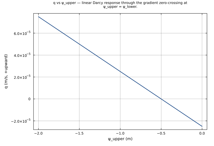
q_vs_psi_upper
Soil water flux vs. upper-layer matric potential at fixed lower-layer state and uniform equilibrium correction. Sweeping ψ_upper from -2.0 m (dry) to 0 m (saturated) at fixed ψ_lower = -0.5 m traces the linear Darcy response of Eq. 5.88: q is positive (upward) when ψ_upper < ψ_lower (capillary rise from wetter lower layer) and negative (downward) when ψ_upper > ψ_lower.
Time span: 0.0 → 1.0
Swept over: ψ_upper
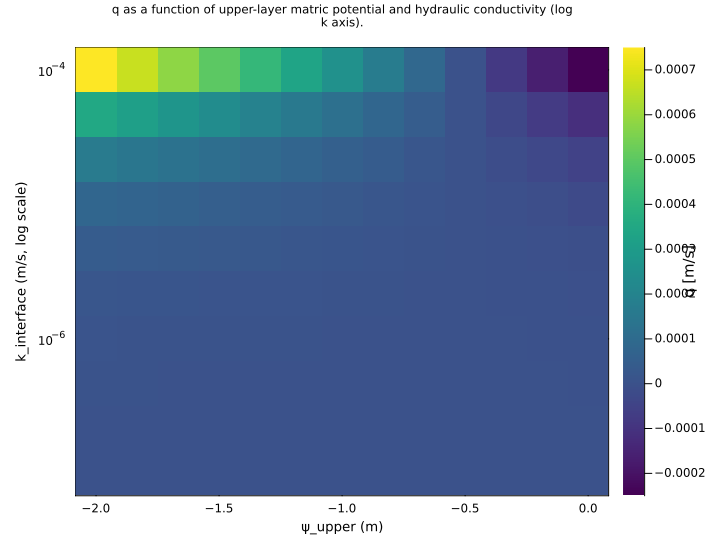
q_vs_psi_upper_and_k
Joint sweep over ψ_upper and k_interface — surfaces the iso-q contours of Eq. 5.88. Higher k_interface amplifies the same matric-potential gradient into proportionally larger fluxes; the iso-q lines are hyperbolae in (ψ_upper, k_interface) space at fixed denominator.
Time span: 0.0 → 1.0
Swept over: ψ_upper, k_interface
Raw .esm
Raw .esm JSON (this component)
{
  "reference": {
    "notes": "source_ref: UrbanCanopy.jl@9200edd4f15609f20339d3a7d104de8064544310:src/hydrology.jl:471\nUpstream `SoilWaterFlux` is an MTK `@component` whose seven inputs (k_interface, ψ_upper, ψ_lower, ψ_E_upper, ψ_E_lower, z_upper, z_lower) are `@parameters` and whose single output (q) is a time-indexed `@variable` with one algebraic equation (Eq. 5.88, no derivative). Identical structure preserved here.\n\nUnicode parameter names ψ_upper, ψ_lower, ψ_E_upper, ψ_E_lower are preserved from upstream — sibling files in this directory (soil_water_content_calc.esm, water_table_depth.esm, interface_hydraulic_conductivity.esm) and components/urban_canopy/temps/freezing_point_depression.esm already established that unicode identifiers are the rig convention for new urban_canopy migrations and the canonical Python runner accepts them.\n\nThe upstream component has no `@constants` block and no defaults in `@parameters`. Defaults here are taken from the upstream Equation Verification test (UrbanCanopy.jl test/hydrology_test.jl:690, equilibrium case): k_interface=1.0e-5 m/s, ψ_upper=-0.5 m, ψ_lower=-1.0 m, ψ_E_upper=-0.3 m, ψ_E_lower=-0.8 m, z_upper=0.1 m, z_lower=0.3 m → q = -1e-5 * ((-0.5-(-1.0)) + (-0.8-(-0.3))) / (0.3-0.1) = -1e-5 * (0.5 + (-0.5)) / 0.2 = 0 m/s. The default state is the canonical equilibrium for which the gravitational-equilibrium correction exactly cancels the matric-potential gradient — a useful default since any non-trivial perturbation surfaces a non-zero flux.\n\nEq. 5.88 form: q = -k[z_h] * [(ψ_i - ψ_{i+1}) + (ψ_{E,i+1} - ψ_{E,i})] / (z_{i+1} - z_i). The bracketed term is the *perturbation* of the matric potential from the local hydrostatic equilibrium (Zeng and Decker 2009) — ψ_E is the equilibrium matric potential at each layer node and ψ - ψ_E is the deviation that drives flux. Without the correction, gravitationally-induced equilibrium gradients would produce a spurious flux; with the correction, the flux vanishes when ψ_upper - ψ_lower = ψ_E_upper - ψ_E_lower (the default scenario).\n\nSign convention: q is positive *upward*. The leading minus sign is encoded in the AST via `{op: '*', args: [-1, k_interface, ...]}`, matching the convention established by sibling files (snow_compaction.esm uses `-1` as a literal first argument to the `*` op).\n\nObservability classification: this component is functionally observed-only — q is given by a single algebraic equation in the parameters (the `(t)` time index has no role since there is no derivative). Test scenarios use `time_span: [0, 1]` and sample at t=0 to mirror the convention used by the other observed-only ESM files in this directory (soil_water_content_calc.esm, water_table_depth.esm, interface_hydraulic_conductivity.esm).\n\nTolerance rationale (model-level rel=1e-9): observed-only algebraic system (no ODE integration); the equation is a chain of three subtractions, one addition, one multiplication (by -1 and k_interface), and one division — eight IEEE-754 float64 operations, worst-case roundoff ~8*ULP ≈ 1e-15. 1e-9 leaves comfortable headroom and is well below any plausible physical-discrimination scale on soil water fluxes (m/s, O(1e-6) for the saturated end and O(1e-12) for the dry end of CLMU soils; gradients across realistic layer separations of O(0.1 m) span ~6 orders of magnitude). Equilibrium / zero-flux tests assert `abs: 1e-15` since the upstream Julia test pins exactly that bound (Eq. 5.88 evaluates to a closed-form zero when the matric-potential perturbation vanishes)."
  },
  "tolerance": {
    "rel": 1e-09
  },
  "variables": {
    "k_interface": {
      "type": "parameter",
      "units": "m/s",
      "default": 1e-05,
      "description": "Hydraulic conductivity at the interface between adjacent layers (Oleson Eq. 5.88)"
    },
    "ψ_upper": {
      "type": "parameter",
      "units": "m",
      "default": -0.5,
      "description": "Soil matric potential of the upper layer (negative by convention, SI m)"
    },
    "ψ_lower": {
      "type": "parameter",
      "units": "m",
      "default": -1.0,
      "description": "Soil matric potential of the lower layer (negative by convention, SI m)"
    },
    "ψ_E_upper": {
      "type": "parameter",
      "units": "m",
      "default": -0.3,
      "description": "Equilibrium matric potential of the upper layer (Zeng and Decker 2009 correction, SI m)"
    },
    "ψ_E_lower": {
      "type": "parameter",
      "units": "m",
      "default": -0.8,
      "description": "Equilibrium matric potential of the lower layer (Zeng and Decker 2009 correction, SI m)"
    },
    "z_upper": {
      "type": "parameter",
      "units": "m",
      "default": 0.1,
      "description": "Node depth of the upper layer (positive downward from surface)"
    },
    "z_lower": {
      "type": "parameter",
      "units": "m",
      "default": 0.3,
      "description": "Node depth of the lower layer (positive downward from surface)"
    },
    "q": {
      "type": "unknown",
      "units": "m/s",
      "description": "Soil water flux at the interface (Oleson Eq. 5.88, positive upward)"
    }
  },
  "equations": [
    {
      "lhs": "q",
      "rhs": {
        "op": "/",
        "args": [
          {
            "op": "*",
            "args": [
              -1,
              "k_interface",
              {
                "op": "+",
                "args": [
                  {
                    "op": "-",
                    "args": [
                      "ψ_upper",
                      "ψ_lower"
                    ]
                  },
                  {
                    "op": "-",
                    "args": [
                      "ψ_E_lower",
                      "ψ_E_upper"
                    ]
                  }
                ]
              }
            ]
          },
          {
            "op": "-",
            "args": [
              "z_lower",
              "z_upper"
            ]
          }
        ]
      }
    }
  ],
  "tests": [
    {
      "id": "equilibrium_zero_flux",
      "description": "Canonical equilibrium case from upstream Equation Verification (UrbanCanopy.jl test/hydrology_test.jl:699): k_interface = 1e-5 m/s, ψ_upper = -0.5 m, ψ_lower = -1.0 m, ψ_E_upper = -0.3 m, ψ_E_lower = -0.8 m, z_upper = 0.1 m, z_lower = 0.3 m. The matric-potential gradient (ψ_upper - ψ_lower = 0.5 m) exactly cancels the equilibrium-potential gradient (ψ_E_lower - ψ_E_upper = -0.5 m), so the Zeng and Decker (2009) perturbation vanishes and q = 0 m/s. Verifies the equilibrium branch of Eq. 5.88 — the primary purpose of the equilibrium-potential correction.",
      "parameter_overrides": {
        "k_interface": 1e-05,
        "ψ_upper": -0.5,
        "ψ_lower": -1.0,
        "ψ_E_upper": -0.3,
        "ψ_E_lower": -0.8,
        "z_upper": 0.1,
        "z_lower": 0.3
      },
      "time_span": {
        "start": 0.0,
        "end": 1.0
      },
      "assertions": [
        {
          "variable": "q",
          "time": 0.0,
          "expected": 0.0,
          "tolerance": {
            "abs": 1e-15
          }
        }
      ]
    },
    {
      "id": "non_zero_downward_flux",
      "description": "Non-zero downward flux from upstream Equation Verification (UrbanCanopy.jl test/hydrology_test.jl:715): k_interface = 1e-5 m/s, ψ_upper = -0.2 m, ψ_lower = -0.5 m, ψ_E_upper = ψ_E_lower = -0.1 m (uniform equilibrium → no correction), z_upper = 0.1 m, z_lower = 0.3 m. The matric-potential perturbation drives flux: q = -1e-5 * ((-0.2 - (-0.5)) + 0) / 0.2 = -1e-5 * 0.3 / 0.2 = -1.5e-5 m/s (negative → downward, consistent with the upper layer being wetter / less negative ψ). Verifies the non-equilibrium branch of Eq. 5.88.",
      "parameter_overrides": {
        "k_interface": 1e-05,
        "ψ_upper": -0.2,
        "ψ_lower": -0.5,
        "ψ_E_upper": -0.1,
        "ψ_E_lower": -0.1,
        "z_upper": 0.1,
        "z_lower": 0.3
      },
      "time_span": {
        "start": 0.0,
        "end": 1.0
      },
      "assertions": [
        {
          "variable": "q",
          "time": 0.0,
          "expected": -1.5e-05
        }
      ]
    },
    {
      "id": "upward_flux_dry_upper",
      "description": "Upward flux: the lower layer is wetter (less negative ψ) than the upper layer, so soil water moves upward to relieve the matric-potential gradient (capillary rise). k_interface = 2e-6 m/s, ψ_upper = -1.5 m, ψ_lower = -0.5 m, uniform equilibrium ψ_E_* = -0.1 m, z_upper = 0.1 m, z_lower = 0.3 m. q = -2e-6 * ((-1.5 - (-0.5)) + 0) / 0.2 = -2e-6 * (-1.0) / 0.2 = +1.0e-5 m/s (positive → upward). Verifies the sign convention (positive upward) and an upward-driven flux.",
      "parameter_overrides": {
        "k_interface": 2e-06,
        "ψ_upper": -1.5,
        "ψ_lower": -0.5,
        "ψ_E_upper": -0.1,
        "ψ_E_lower": -0.1,
        "z_upper": 0.1,
        "z_lower": 0.3
      },
      "time_span": {
        "start": 0.0,
        "end": 1.0
      },
      "assertions": [
        {
          "variable": "q",
          "time": 0.0,
          "expected": 1e-05
        }
      ]
    },
    {
      "id": "pure_equilibrium_perturbation",
      "description": "Pure equilibrium-perturbation flux: the matric potentials are uniform (ψ_upper = ψ_lower) so the actual gradient is zero, but the equilibrium potentials differ. q is driven entirely by the (ψ_E_lower - ψ_E_upper) term. k_interface = 1e-5 m/s, ψ_upper = ψ_lower = -0.5 m, ψ_E_upper = -0.4 m, ψ_E_lower = -0.6 m, z_upper = 0.1 m, z_lower = 0.3 m. q = -1e-5 * (0 + (-0.6 - (-0.4))) / 0.2 = -1e-5 * (-0.2) / 0.2 = +1.0e-5 m/s. Isolates the Zeng-Decker correction term and confirms its sign convention.",
      "parameter_overrides": {
        "k_interface": 1e-05,
        "ψ_upper": -0.5,
        "ψ_lower": -0.5,
        "ψ_E_upper": -0.4,
        "ψ_E_lower": -0.6,
        "z_upper": 0.1,
        "z_lower": 0.3
      },
      "time_span": {
        "start": 0.0,
        "end": 1.0
      },
      "assertions": [
        {
          "variable": "q",
          "time": 0.0,
          "expected": 1e-05
        }
      ]
    },
    {
      "id": "wider_layer_separation",
      "description": "Wider layer separation reduces the gradient and so reduces |q| at fixed potentials. Same matric and equilibrium potentials as `non_zero_downward_flux`, but z_lower = 1.1 m instead of 0.3 m so (z_lower - z_upper) = 1.0 m (5× larger). q = -1e-5 * 0.3 / 1.0 = -3.0e-6 m/s, i.e. 5× smaller magnitude than the canonical 0.3 m separation case. Exercises the 1/(z_lower - z_upper) dependence in Eq. 5.88.",
      "parameter_overrides": {
        "k_interface": 1e-05,
        "ψ_upper": -0.2,
        "ψ_lower": -0.5,
        "ψ_E_upper": -0.1,
        "ψ_E_lower": -0.1,
        "z_upper": 0.1,
        "z_lower": 1.1
      },
      "time_span": {
        "start": 0.0,
        "end": 1.0
      },
      "assertions": [
        {
          "variable": "q",
          "time": 0.0,
          "expected": -3e-06
        }
      ]
    },
    {
      "id": "high_conductivity_proportional",
      "description": "Flux is linearly proportional to k_interface. With the same `non_zero_downward_flux` potentials and geometry but k_interface = 1e-4 m/s (10× larger), q = -1e-4 * 0.3 / 0.2 = -1.5e-4 m/s (10× larger magnitude). Exercises the linear k_interface scaling in Eq. 5.88 — important since k_interface itself varies over many orders of magnitude across the soil saturation range (~1e-12 to ~1e-5 m/s).",
      "parameter_overrides": {
        "k_interface": 0.0001,
        "ψ_upper": -0.2,
        "ψ_lower": -0.5,
        "ψ_E_upper": -0.1,
        "ψ_E_lower": -0.1,
        "z_upper": 0.1,
        "z_lower": 0.3
      },
      "time_span": {
        "start": 0.0,
        "end": 1.0
      },
      "assertions": [
        {
          "variable": "q",
          "time": 0.0,
          "expected": -0.00015
        }
      ]
    },
    {
      "id": "zero_conductivity_zero_flux",
      "description": "Zero hydraulic conductivity (e.g. fully frozen layer, k_interface → 0) blocks all flux regardless of the matric-potential gradient. k_interface = 0.0, all other parameters from the `non_zero_downward_flux` scenario. q = 0 * (anything) / (anything > 0) = 0 m/s. Verifies the k_interface = 0 limit of Eq. 5.88 — physically meaningful for frozen or impervious interfaces.",
      "parameter_overrides": {
        "k_interface": 0.0,
        "ψ_upper": -0.2,
        "ψ_lower": -0.5,
        "ψ_E_upper": -0.1,
        "ψ_E_lower": -0.1,
        "z_upper": 0.1,
        "z_lower": 0.3
      },
      "time_span": {
        "start": 0.0,
        "end": 1.0
      },
      "assertions": [
        {
          "variable": "q",
          "time": 0.0,
          "expected": 0.0,
          "tolerance": {
            "abs": 1e-15
          }
        }
      ]
    },
    {
      "id": "deep_soil_low_conductivity",
      "description": "Deep soil column with low conductivity and a small matric-potential gradient — representative of a near-saturation interior layer pair. k_interface = 5e-8 m/s, ψ_upper = -2.0 m, ψ_lower = -2.1 m (small gradient), uniform equilibrium ψ_E_* = -1.0 m, z_upper = 1.5 m, z_lower = 2.0 m (deep interface, 0.5 m separation). q = -5e-8 * ((-2.0 - (-2.1)) + 0) / 0.5 = -5e-8 * 0.1 / 0.5 = -1.0e-8 m/s. Tests Eq. 5.88 at a small-magnitude operating point characteristic of the deep mineral-soil column.",
      "parameter_overrides": {
        "k_interface": 5e-08,
        "ψ_upper": -2.0,
        "ψ_lower": -2.1,
        "ψ_E_upper": -1.0,
        "ψ_E_lower": -1.0,
        "z_upper": 1.5,
        "z_lower": 2.0
      },
      "time_span": {
        "start": 0.0,
        "end": 1.0
      },
      "assertions": [
        {
          "variable": "q",
          "time": 0.0,
          "expected": -1e-08
        }
      ]
    }
  ],
  "analyses": [
    {
      "id": "q_vs_psi_upper",
      "description": "Soil water flux vs. upper-layer matric potential at fixed lower-layer state and uniform equilibrium correction. Sweeping ψ_upper from -2.0 m (dry) to 0 m (saturated) at fixed ψ_lower = -0.5 m traces the linear Darcy response of Eq. 5.88: q is positive (upward) when ψ_upper < ψ_lower (capillary rise from wetter lower layer) and negative (downward) when ψ_upper > ψ_lower.",
      "initial_state": {},
      "parameters": {
        "k_interface": 1e-05,
        "ψ_lower": -0.5,
        "ψ_E_upper": -0.1,
        "ψ_E_lower": -0.1,
        "z_upper": 0.1,
        "z_lower": 0.3
      },
      "time_span": {
        "start": 0.0,
        "end": 1.0
      },
      "parameter_sweep": {
        "type": "cartesian",
        "dimensions": [
          {
            "parameter": "ψ_upper",
            "range": {
              "start": -2.0,
              "stop": 0.0,
              "count": 21,
              "scale": "linear"
            }
          }
        ]
      },
      "plots": [
        {
          "id": "q_vs_psi_upper_line",
          "type": "line",
          "description": "q vs ψ_upper — linear Darcy response through the gradient zero-crossing at ψ_upper = ψ_lower.",
          "x": {
            "variable": "ψ_upper",
            "label": "ψ_upper (m)"
          },
          "y": {
            "variable": "q",
            "label": "q (m/s, +upward)"
          }
        }
      ]
    },
    {
      "id": "q_vs_psi_upper_and_k",
      "description": "Joint sweep over ψ_upper and k_interface — surfaces the iso-q contours of Eq. 5.88. Higher k_interface amplifies the same matric-potential gradient into proportionally larger fluxes; the iso-q lines are hyperbolae in (ψ_upper, k_interface) space at fixed denominator.",
      "initial_state": {},
      "parameters": {
        "ψ_lower": -0.5,
        "ψ_E_upper": -0.1,
        "ψ_E_lower": -0.1,
        "z_upper": 0.1,
        "z_lower": 0.3
      },
      "time_span": {
        "start": 0.0,
        "end": 1.0
      },
      "parameter_sweep": {
        "type": "cartesian",
        "dimensions": [
          {
            "parameter": "ψ_upper",
            "range": {
              "start": -2.0,
              "stop": 0.0,
              "count": 13,
              "scale": "linear"
            }
          },
          {
            "parameter": "k_interface",
            "range": {
              "start": 1e-07,
              "stop": 0.0001,
              "count": 10,
              "scale": "log"
            }
          }
        ]
      },
      "plots": [
        {
          "id": "q_heatmap",
          "type": "heatmap",
          "description": "q as a function of upper-layer matric potential and hydraulic conductivity (log k axis).",
          "x": {
            "variable": "ψ_upper",
            "label": "ψ_upper (m)"
          },
          "y": {
            "variable": "k_interface",
            "label": "k_interface (m/s, log scale)"
          },
          "value": {
            "variable": "q",
            "reduce": "final"
          }
        }
      ]
    }
  ]
}