InterfaceHydraulicConductivity
Hydraulic conductivity at a soil-layer interface as a Clapp-Hornberger function of the average volumetric water content and porosity of the two adjacent layers, scaled by the unfrozen fraction. Implements Oleson et al. (2010, CLM Tech Note Ch. 5) Eq. 5.69 (interface conductivity) with the frozen-fraction multiplier of Eq. 5.70. Migrated from UrbanCanopy.jl@9200edd4 src/hydrology.jl:1053 (`InterfaceHydraulicConductivity` @component). Observed-only: all eight inputs are parameters and k_h is given by a single algebraic equation.
Description
Hydraulic conductivity at a soil-layer interface as a Clapp-Hornberger function of the average volumetric water content and porosity of the two adjacent layers, scaled by the unfrozen fraction. Implements Oleson et al. (2010, CLM Tech Note Ch. 5) Eq. 5.69 (interface conductivity) with the frozen-fraction multiplier of Eq. 5.70. Migrated from UrbanCanopy.jl@9200edd4 src/hydrology.jl:1053 (InterfaceHydraulicConductivity @component). Observed-only: all eight inputs are parameters and k_h is given by a single algebraic equation.
Reference
_source_ref: UrbanCanopy.jl@9200edd4f15609f20339d3a7d104de8064544310:src/hydrology.jl:1053
Upstream InterfaceHydraulicConductivity is an MTK @component whose eight inputs (k_sat_h, θ_upper, θ_lower, θ_sat_upper, θ_sat_lower, B_i, f_frz_upper, f_frz_lower) are all @parameters and whose single output (k_h) is a time-indexed @variable with one algebraic equation. Identical structure preserved here.
The explicit 0.5 * factors on numerator and denominator (averages of upper/lower water content and porosity) are kept verbatim to mirror the upstream expression — they cancel mathematically but the intent in Oleson Eq. 5.69 is (θ̄ / θ̄_sat), the ratio of arithmetic means of the two layers’ water content and porosity.
The Clapp-Hornberger exponent 2*B + 3 is the standard hydraulic-conductivity exponent for the Clapp-Hornberger (1978) curve as used in Oleson Eq. 5.69. The frozen-fraction multiplier (1 - (f_frz_upper + f_frz_lower)/2) reduces conductivity in proportion to the mean impermeable fraction of the two layers (Oleson Eq. 5.70).
Unicode θ_upper, θ_lower, θ_sat_upper, θ_sat_lower are preserved from upstream — sibling files in this directory (snow_compaction.esm, snow_layer_combination.esm, soil_water_content_calc.esm) already established that unicode identifiers are the rig convention for new urban_canopy migrations and the canonical Python runner accepts them.
Observability classification: this component is functionally observed-only — k_h is given by a single algebraic equation in the parameters. The (t) time index has no role since there is no derivative. Test scenarios use time_span: [0, 1] and sample at t=0 to mirror the convention used by the other observed-only ESM files in this directory (soil_water_content_calc.esm, snow_density.esm).
Default parameter values: k_sat_h = 1.0e-5 m/s and B_i = 6.0 are the canonical mid-range Clapp-Hornberger parameters used in the upstream test fixtures (UrbanCanopy.jl test/hydrology_test.jl:1310). Default θ_sat = 0.4 m^3/m^3 is a typical CLMU mineral-soil porosity. Default θ values are set to θ_sat (saturated layer) so that the no-override default scenario evaluates to k_h = k_sat_h, matching the saturation limit of Eq. 5.69. f_frz defaults are 0 (unfrozen).
Tolerance rationale (model-level rel=1e-9): observed-only algebraic system (no ODE integration); the equation involves O(10) IEEE-754 float64 operations including a 15th-power exponentiation in the canonical fixture, so worst-case roundoff is ~10*ULP * (a few extra ULPs from pow) ≈ 1e-13. 1e-9 leaves comfortable headroom and is well below any plausible physical-discrimination scale on hydraulic conductivity (which spans ~10 orders of magnitude across saturated→dry soils). The fully-frozen case asserts an exact algebraic zero (abs: 1e-15) since the frozen multiplier yields a hard zero independent of the exponent value._
Parameters
| Name | Units | Default | Description |
|---|---|---|---|
k_sat_h | m/s | 1e-05 | Saturated hydraulic conductivity at interface (Eq. 5.70) |
θ_upper | m^3/m^3 | 0.4 | Volumetric water content of upper layer |
θ_lower | m^3/m^3 | 0.4 | Volumetric water content of lower layer |
θ_sat_upper | m^3/m^3 | 0.4 | Porosity of upper layer |
θ_sat_lower | m^3/m^3 | 0.4 | Porosity of lower layer |
B_i | 1 | 6.0 | Clapp-Hornberger exponent of upper layer (dimensionless) |
f_frz_upper | 1 | 0.0 | Impermeable fraction of upper layer (dimensionless) |
f_frz_lower | 1 | 0.0 | Impermeable fraction of lower layer (dimensionless) |
Observed
| Name | Units | Default | Description |
|---|---|---|---|
k_h | m/s | Hydraulic conductivity at interface (Oleson Eq. 5.69 with Eq. 5.70 frozen-fraction reduction) |
Observed expressions
$$ k_{h} = \left(1.0 - \frac{f_{frz\,upper} + f_{frz\,lower}}{2.0}\right) \cdot k_{sat\,h} \cdot \frac{0.5 \cdot \left(θ_{upper} + θ_{lower}\right)}{0.5 \cdot \left(θ_{sat\,upper} + θ_{sat\,lower}\right)}^{2.0 \cdot B_{i} + 3.0} $$Hydraulic conductivity at interface (Oleson Eq. 5.69 with Eq. 5.70 frozen-fraction reduction)
Analyses
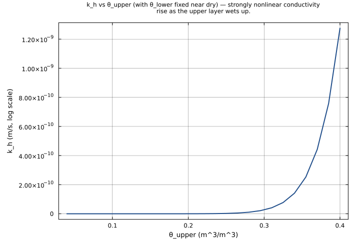
k_h_vs_saturation
Hydraulic conductivity vs. degree of saturation S = θ/θ_sat for the canonical Clapp-Hornberger exponent B = 6. Reproduces the upstream documentation plot (UrbanCanopy.jl docs/src/hydrology.md, ‘Interface Hydraulic Conductivity vs Saturation’). Sweeps θ from near-dry to saturation at fixed θ_sat = 0.4 — the strongly nonlinear k_h(S) ∝ S^15 dependence is the dominant feature of Eq. 5.69.
Time span: 0.0 → 1.0
Swept over: θ_upper
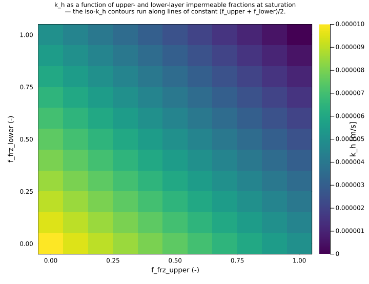
k_h_vs_freezing
Hydraulic conductivity vs. mean impermeable fraction at saturation. Layers are at θ = θ_sat = 0.4 so the conductivity ratio is 1; the (1 - mean f_frz) multiplier of Eq. 5.70 then drives k_h linearly from k_sat_h at f = 0 to 0 at f = 1. Equal upper/lower fractions are swept jointly to reproduce the upstream qualitative-behavior test (UrbanCanopy.jl test/hydrology_test.jl:1348).
Time span: 0.0 → 1.0
Swept over: f_frz_upper, f_frz_lower
Raw .esm
Raw .esm JSON (this component)
{
  "reference": {
    "notes": "source_ref: UrbanCanopy.jl@9200edd4f15609f20339d3a7d104de8064544310:src/hydrology.jl:1053\nUpstream `InterfaceHydraulicConductivity` is an MTK `@component` whose eight inputs (k_sat_h, θ_upper, θ_lower, θ_sat_upper, θ_sat_lower, B_i, f_frz_upper, f_frz_lower) are all `@parameters` and whose single output (k_h) is a time-indexed `@variable` with one algebraic equation. Identical structure preserved here.\n\nThe explicit `0.5 *` factors on numerator and denominator (averages of upper/lower water content and porosity) are kept verbatim to mirror the upstream expression — they cancel mathematically but the intent in Oleson Eq. 5.69 is `(θ̄ / θ̄_sat)`, the ratio of arithmetic means of the two layers' water content and porosity.\n\nThe Clapp-Hornberger exponent `2*B + 3` is the standard hydraulic-conductivity exponent for the Clapp-Hornberger (1978) curve as used in Oleson Eq. 5.69. The frozen-fraction multiplier `(1 - (f_frz_upper + f_frz_lower)/2)` reduces conductivity in proportion to the mean impermeable fraction of the two layers (Oleson Eq. 5.70).\n\nUnicode `θ_upper`, `θ_lower`, `θ_sat_upper`, `θ_sat_lower` are preserved from upstream — sibling files in this directory (snow_compaction.esm, snow_layer_combination.esm, soil_water_content_calc.esm) already established that unicode identifiers are the rig convention for new urban_canopy migrations and the canonical Python runner accepts them.\n\nObservability classification: this component is functionally observed-only — k_h is given by a single algebraic equation in the parameters. The `(t)` time index has no role since there is no derivative. Test scenarios use `time_span: [0, 1]` and sample at t=0 to mirror the convention used by the other observed-only ESM files in this directory (soil_water_content_calc.esm, snow_density.esm).\n\nDefault parameter values: k_sat_h = 1.0e-5 m/s and B_i = 6.0 are the canonical mid-range Clapp-Hornberger parameters used in the upstream test fixtures (UrbanCanopy.jl test/hydrology_test.jl:1310). Default θ_sat = 0.4 m^3/m^3 is a typical CLMU mineral-soil porosity. Default θ values are set to θ_sat (saturated layer) so that the no-override default scenario evaluates to k_h = k_sat_h, matching the saturation limit of Eq. 5.69. f_frz defaults are 0 (unfrozen).\n\nTolerance rationale (model-level rel=1e-9): observed-only algebraic system (no ODE integration); the equation involves O(10) IEEE-754 float64 operations including a 15th-power exponentiation in the canonical fixture, so worst-case roundoff is ~10*ULP * (a few extra ULPs from `pow`) ≈ 1e-13. 1e-9 leaves comfortable headroom and is well below any plausible physical-discrimination scale on hydraulic conductivity (which spans ~10 orders of magnitude across saturated→dry soils). The fully-frozen case asserts an exact algebraic zero (`abs: 1e-15`) since the frozen multiplier yields a hard zero independent of the exponent value."
  },
  "tolerance": {
    "rel": 1e-09
  },
  "variables": {
    "k_sat_h": {
      "type": "parameter",
      "units": "m/s",
      "default": 1e-05,
      "description": "Saturated hydraulic conductivity at interface (Eq. 5.70)"
    },
    "θ_upper": {
      "type": "parameter",
      "units": "m^3/m^3",
      "default": 0.4,
      "description": "Volumetric water content of upper layer"
    },
    "θ_lower": {
      "type": "parameter",
      "units": "m^3/m^3",
      "default": 0.4,
      "description": "Volumetric water content of lower layer"
    },
    "θ_sat_upper": {
      "type": "parameter",
      "units": "m^3/m^3",
      "default": 0.4,
      "description": "Porosity of upper layer"
    },
    "θ_sat_lower": {
      "type": "parameter",
      "units": "m^3/m^3",
      "default": 0.4,
      "description": "Porosity of lower layer"
    },
    "B_i": {
      "type": "parameter",
      "units": "1",
      "default": 6.0,
      "description": "Clapp-Hornberger exponent of upper layer (dimensionless)"
    },
    "f_frz_upper": {
      "type": "parameter",
      "units": "1",
      "default": 0.0,
      "description": "Impermeable fraction of upper layer (dimensionless)"
    },
    "f_frz_lower": {
      "type": "parameter",
      "units": "1",
      "default": 0.0,
      "description": "Impermeable fraction of lower layer (dimensionless)"
    },
    "k_h": {
      "type": "unknown",
      "units": "m/s",
      "description": "Hydraulic conductivity at interface (Oleson Eq. 5.69 with Eq. 5.70 frozen-fraction reduction)"
    }
  },
  "equations": [
    {
      "lhs": "k_h",
      "rhs": {
        "op": "*",
        "args": [
          {
            "op": "-",
            "args": [
              1.0,
              {
                "op": "/",
                "args": [
                  {
                    "op": "+",
                    "args": [
                      "f_frz_upper",
                      "f_frz_lower"
                    ]
                  },
                  2.0
                ]
              }
            ]
          },
          "k_sat_h",
          {
            "op": "^",
            "args": [
              {
                "op": "/",
                "args": [
                  {
                    "op": "*",
                    "args": [
                      0.5,
                      {
                        "op": "+",
                        "args": [
                          "θ_upper",
                          "θ_lower"
                        ]
                      }
                    ]
                  },
                  {
                    "op": "*",
                    "args": [
                      0.5,
                      {
                        "op": "+",
                        "args": [
                          "θ_sat_upper",
                          "θ_sat_lower"
                        ]
                      }
                    ]
                  }
                ]
              },
              {
                "op": "+",
                "args": [
                  {
                    "op": "*",
                    "args": [
                      2.0,
                      "B_i"
                    ]
                  },
                  3.0
                ]
              }
            ]
          }
        ]
      }
    }
  ],
  "tests": [
    {
      "id": "saturated_no_freeze",
      "description": "Saturation limit of Eq. 5.69 with no freezing: θ_upper = θ_lower = θ_sat = 0.4 m^3/m^3, B_i = 6, f_frz = 0. The conductivity ratio is (0.4/0.4)^15 = 1 and the unfrozen multiplier is 1, so k_h reduces to k_sat_h = 1e-5 m/s. Verifies the canonical saturation limit (mirrors UrbanCanopy.jl test/hydrology_test.jl:1310 'Test 1').",
      "parameter_overrides": {
        "k_sat_h": 1e-05,
        "θ_upper": 0.4,
        "θ_lower": 0.4,
        "θ_sat_upper": 0.4,
        "θ_sat_lower": 0.4,
        "B_i": 6.0,
        "f_frz_upper": 0.0,
        "f_frz_lower": 0.0
      },
      "time_span": {
        "start": 0.0,
        "end": 1.0
      },
      "assertions": [
        {
          "variable": "k_h",
          "time": 0.0,
          "expected": 1e-05
        }
      ]
    },
    {
      "id": "half_saturation_no_freeze",
      "description": "Half-saturation case: θ_upper = θ_lower = 0.2, θ_sat = 0.4, B_i = 6, f_frz = 0. k_h = k_sat_h * 0.5^(2*6+3) = 1e-5 * 0.5^15 = 1e-5 * 3.0517578125e-5 ≈ 3.0518e-10 m/s. Exercises the strong nonlinearity of the Clapp-Hornberger exponent — a 2× drop in θ at B=6 reduces conductivity by 5 orders of magnitude (mirrors UrbanCanopy.jl 'Test 2').",
      "parameter_overrides": {
        "k_sat_h": 1e-05,
        "θ_upper": 0.2,
        "θ_lower": 0.2,
        "θ_sat_upper": 0.4,
        "θ_sat_lower": 0.4,
        "B_i": 6.0,
        "f_frz_upper": 0.0,
        "f_frz_lower": 0.0
      },
      "time_span": {
        "start": 0.0,
        "end": 1.0
      },
      "assertions": [
        {
          "variable": "k_h",
          "time": 0.0,
          "expected": 3.0517578125e-10
        }
      ]
    },
    {
      "id": "fully_frozen",
      "description": "Full-freezing limit: f_frz_upper = f_frz_lower = 1, layers otherwise saturated. The (1 - (f_upper+f_lower)/2) multiplier of Eq. 5.70 is exactly zero, so k_h = 0 regardless of any other parameter — exercises the hard-cutoff behavior of the frozen-fraction reduction (mirrors UrbanCanopy.jl 'Test 3'). Asserted at IEEE-754 zero (abs=1e-15).",
      "parameter_overrides": {
        "k_sat_h": 1e-05,
        "θ_upper": 0.4,
        "θ_lower": 0.4,
        "θ_sat_upper": 0.4,
        "θ_sat_lower": 0.4,
        "B_i": 6.0,
        "f_frz_upper": 1.0,
        "f_frz_lower": 1.0
      },
      "time_span": {
        "start": 0.0,
        "end": 1.0
      },
      "assertions": [
        {
          "variable": "k_h",
          "time": 0.0,
          "expected": 0.0,
          "tolerance": {
            "abs": 1e-15
          }
        }
      ]
    },
    {
      "id": "half_frozen_at_saturation",
      "description": "Partial freezing at saturation: f_frz_upper = f_frz_lower = 0.5, θ at saturation. The frozen-fraction multiplier is 1 - 0.5 = 0.5 and the conductivity ratio is 1, so k_h = 0.5 * k_sat_h = 5e-6 m/s. Verifies that the linear frozen-fraction reduction of Eq. 5.70 is correctly applied (mirrors UrbanCanopy.jl 'Test 4').",
      "parameter_overrides": {
        "k_sat_h": 1e-05,
        "θ_upper": 0.4,
        "θ_lower": 0.4,
        "θ_sat_upper": 0.4,
        "θ_sat_lower": 0.4,
        "B_i": 6.0,
        "f_frz_upper": 0.5,
        "f_frz_lower": 0.5
      },
      "time_span": {
        "start": 0.0,
        "end": 1.0
      },
      "assertions": [
        {
          "variable": "k_h",
          "time": 0.0,
          "expected": 5e-06
        }
      ]
    },
    {
      "id": "quarter_saturation_low_B",
      "description": "Quarter-saturation with a low Clapp-Hornberger exponent: θ = 0.1, θ_sat = 0.4, B_i = 3 (sandy soil). k_h = 1e-5 * 0.25^9 = 1e-5 * 3.814697e-6 ≈ 3.815e-11 m/s. Exercises a different B regime where the exponent (2*3+3 = 9) is roughly half the canonical 15 — the dependence on B is the dominant lever in Eq. 5.69.",
      "parameter_overrides": {
        "k_sat_h": 1e-05,
        "θ_upper": 0.1,
        "θ_lower": 0.1,
        "θ_sat_upper": 0.4,
        "θ_sat_lower": 0.4,
        "B_i": 3.0,
        "f_frz_upper": 0.0,
        "f_frz_lower": 0.0
      },
      "time_span": {
        "start": 0.0,
        "end": 1.0
      },
      "assertions": [
        {
          "variable": "k_h",
          "time": 0.0,
          "expected": 3.814697265625e-11
        }
      ]
    },
    {
      "id": "asymmetric_water_content",
      "description": "Layer-asymmetric water content: θ_upper = 0.3, θ_lower = 0.1, θ_sat_upper = θ_sat_lower = 0.4. The arithmetic-mean numerator is 0.5*(0.3+0.1) = 0.2 (same as half-saturation case) so k_h ≈ 3.0518e-10 m/s — exercises the averaging behavior of the interface formulation (the conductivity is a function of mean water content, not of either layer individually).",
      "parameter_overrides": {
        "k_sat_h": 1e-05,
        "θ_upper": 0.3,
        "θ_lower": 0.1,
        "θ_sat_upper": 0.4,
        "θ_sat_lower": 0.4,
        "B_i": 6.0,
        "f_frz_upper": 0.0,
        "f_frz_lower": 0.0
      },
      "time_span": {
        "start": 0.0,
        "end": 1.0
      },
      "assertions": [
        {
          "variable": "k_h",
          "time": 0.0,
          "expected": 3.0517578125e-10
        }
      ]
    },
    {
      "id": "heterogeneous_porosities",
      "description": "Layer-heterogeneous porosity: θ_upper = θ_lower = 0.3, θ_sat_upper = 0.5, θ_sat_lower = 0.3. The mean θ is 0.3 and the mean θ_sat is 0.4, so the saturation ratio is 0.75. k_h = 1e-5 * 0.75^15 ≈ 1.336e-7 m/s. Verifies that the formulation correctly uses the *averaged* porosity in the denominator (a sand-over-clay column where the upper layer is more porous than the lower).",
      "parameter_overrides": {
        "k_sat_h": 1e-05,
        "θ_upper": 0.3,
        "θ_lower": 0.3,
        "θ_sat_upper": 0.5,
        "θ_sat_lower": 0.3,
        "B_i": 6.0,
        "f_frz_upper": 0.0,
        "f_frz_lower": 0.0
      },
      "time_span": {
        "start": 0.0,
        "end": 1.0
      },
      "assertions": [
        {
          "variable": "k_h",
          "time": 0.0,
          "expected": 1.3363461010158033e-07
        }
      ]
    },
    {
      "id": "asymmetric_freezing",
      "description": "One layer unfrozen, one half-frozen: f_frz_upper = 0, f_frz_lower = 0.5, layers otherwise saturated. The mean-impermeable-fraction multiplier is 1 - 0.25 = 0.75, so k_h = 0.75 * 1e-5 = 7.5e-6 m/s. Verifies that the frozen-fraction multiplier of Eq. 5.70 averages the two layers' impermeable fractions linearly (typical autumn freeze-front state where only one of the two layers has frozen).",
      "parameter_overrides": {
        "k_sat_h": 1e-05,
        "θ_upper": 0.4,
        "θ_lower": 0.4,
        "θ_sat_upper": 0.4,
        "θ_sat_lower": 0.4,
        "B_i": 6.0,
        "f_frz_upper": 0.0,
        "f_frz_lower": 0.5
      },
      "time_span": {
        "start": 0.0,
        "end": 1.0
      },
      "assertions": [
        {
          "variable": "k_h",
          "time": 0.0,
          "expected": 7.500000000000001e-06
        }
      ]
    },
    {
      "id": "high_B_partial_saturation",
      "description": "High Clapp-Hornberger exponent (B_i = 10, characteristic of a heavy clay) at partial saturation θ/θ_sat = 0.75. The exponent is 2*10+3 = 23, so k_h = 1e-5 * 0.75^23 ≈ 1.338e-8 m/s. Stress-tests the exponentiation pathway at a large exponent (high-B clays exhibit the steepest conductivity drop with desaturation).",
      "parameter_overrides": {
        "k_sat_h": 1e-05,
        "θ_upper": 0.3,
        "θ_lower": 0.3,
        "θ_sat_upper": 0.4,
        "θ_sat_lower": 0.4,
        "B_i": 10.0,
        "f_frz_upper": 0.0,
        "f_frz_lower": 0.0
      },
      "time_span": {
        "start": 0.0,
        "end": 1.0
      },
      "assertions": [
        {
          "variable": "k_h",
          "time": 0.0,
          "expected": 1.337855036737774e-08
        }
      ]
    },
    {
      "id": "typical_clmu_unfrozen",
      "description": "Realistic CLMU mid-column unfrozen state: k_sat_h = 2.5e-6 m/s (loamy soil), θ_upper = 0.25, θ_lower = 0.20, θ_sat = 0.45, B_i = 7. Mean θ = 0.225, ratio = 0.5, exponent = 17. k_h = 2.5e-6 * 0.5^17 ≈ 1.907e-11 m/s. Represents a typical drying-front state where the column is at half saturation and the conductivity has dropped 5 orders of magnitude below its saturated value.",
      "parameter_overrides": {
        "k_sat_h": 2.5e-06,
        "θ_upper": 0.25,
        "θ_lower": 0.2,
        "θ_sat_upper": 0.45,
        "θ_sat_lower": 0.45,
        "B_i": 7.0,
        "f_frz_upper": 0.0,
        "f_frz_lower": 0.0
      },
      "time_span": {
        "start": 0.0,
        "end": 1.0
      },
      "assertions": [
        {
          "variable": "k_h",
          "time": 0.0,
          "expected": 1.9073486328125e-11
        }
      ]
    }
  ],
  "analyses": [
    {
      "id": "k_h_vs_saturation",
      "description": "Hydraulic conductivity vs. degree of saturation S = θ/θ_sat for the canonical Clapp-Hornberger exponent B = 6. Reproduces the upstream documentation plot (UrbanCanopy.jl docs/src/hydrology.md, 'Interface Hydraulic Conductivity vs Saturation'). Sweeps θ from near-dry to saturation at fixed θ_sat = 0.4 — the strongly nonlinear k_h(S) ∝ S^15 dependence is the dominant feature of Eq. 5.69.",
      "initial_state": {},
      "parameters": {
        "k_sat_h": 1e-05,
        "θ_sat_upper": 0.4,
        "θ_sat_lower": 0.4,
        "B_i": 6.0,
        "f_frz_upper": 0.0,
        "f_frz_lower": 0.0,
        "θ_lower": 0.04
      },
      "time_span": {
        "start": 0.0,
        "end": 1.0
      },
      "parameter_sweep": {
        "type": "cartesian",
        "dimensions": [
          {
            "parameter": "θ_upper",
            "range": {
              "start": 0.04,
              "stop": 0.4,
              "count": 25,
              "scale": "linear"
            }
          }
        ]
      },
      "plots": [
        {
          "id": "k_h_vs_theta",
          "type": "line",
          "description": "k_h vs θ_upper (with θ_lower fixed near dry) — strongly nonlinear conductivity rise as the upper layer wets up.",
          "x": {
            "variable": "θ_upper",
            "label": "θ_upper (m^3/m^3)"
          },
          "y": {
            "variable": "k_h",
            "label": "k_h (m/s, log scale)"
          }
        }
      ]
    },
    {
      "id": "k_h_vs_freezing",
      "description": "Hydraulic conductivity vs. mean impermeable fraction at saturation. Layers are at θ = θ_sat = 0.4 so the conductivity ratio is 1; the (1 - mean f_frz) multiplier of Eq. 5.70 then drives k_h linearly from k_sat_h at f = 0 to 0 at f = 1. Equal upper/lower fractions are swept jointly to reproduce the upstream qualitative-behavior test (UrbanCanopy.jl test/hydrology_test.jl:1348).",
      "initial_state": {},
      "parameters": {
        "k_sat_h": 1e-05,
        "θ_upper": 0.4,
        "θ_lower": 0.4,
        "θ_sat_upper": 0.4,
        "θ_sat_lower": 0.4,
        "B_i": 6.0
      },
      "time_span": {
        "start": 0.0,
        "end": 1.0
      },
      "parameter_sweep": {
        "type": "cartesian",
        "dimensions": [
          {
            "parameter": "f_frz_upper",
            "range": {
              "start": 0.0,
              "stop": 1.0,
              "count": 11,
              "scale": "linear"
            }
          },
          {
            "parameter": "f_frz_lower",
            "range": {
              "start": 0.0,
              "stop": 1.0,
              "count": 11,
              "scale": "linear"
            }
          }
        ]
      },
      "plots": [
        {
          "id": "k_h_freezing_heatmap",
          "type": "heatmap",
          "description": "k_h as a function of upper- and lower-layer impermeable fractions at saturation — the iso-k_h contours run along lines of constant (f_upper + f_lower)/2.",
          "x": {
            "variable": "f_frz_upper",
            "label": "f_frz_upper (-)"
          },
          "y": {
            "variable": "f_frz_lower",
            "label": "f_frz_lower (-)"
          },
          "value": {
            "variable": "k_h",
            "reduce": "final"
          }
        }
      ]
    }
  ]
}