PlanetaryEnergyBalance
Planetary equilibrium temperature from the top-of-atmosphere energy balance (Seinfeld & Pandis 2006 Ch. 4 Eqs. 4.5-4.7). The absorbed solar flux F_S = S_0/4 * (1 - R_p), the emitted longwave flux F_L = sigma * T_e^4 (Stefan-Boltzmann law), and at equilibrium F_S = F_L. Solving the constraint gives T_e = (S_0/4 * (1-R_p) / sigma)^(1/4). At canonical Earth values (S_0 = 1370 W/m^2, R_p = 0.3), F_S = F_L = 239.75 W/m^2 and T_e = 255 K (S&P p. 101). Migrated from GasChem.jl@8c12c048 src/radiation_fundamentals.jl:211 (`PlanetaryEnergyBalance` @component).
Description
Planetary equilibrium temperature from the top-of-atmosphere energy balance (Seinfeld & Pandis 2006 Ch. 4 Eqs. 4.5-4.7). The absorbed solar flux F_S = S_0/4 * (1 - R_p), the emitted longwave flux F_L = sigma * T_e^4 (Stefan-Boltzmann law), and at equilibrium F_S = F_L. Solving the constraint gives T_e = (S_0/4 * (1-R_p) / sigma)^(1/4). At canonical Earth values (S_0 = 1370 W/m^2, R_p = 0.3), F_S = F_L = 239.75 W/m^2 and T_e = 255 K (S&P p. 101). Migrated from GasChem.jl@8c12c048 src/radiation_fundamentals.jl:211 (PlanetaryEnergyBalance @component).
Reference
_source_ref: GasChem.jl@8c12c048482b515fb8eb2110bf8ab4b4f4e71309:src/radiation_fundamentals.jl:211
Upstream PlanetaryEnergyBalance is an MTK @component with one @constants block (sigma = 5.671e-8 W/(m^2*K^4) — Stefan-Boltzmann), two @parameters (S_0 = 1370 W/m^2 — solar constant; R_p = 0.3 — planetary albedo), three time-indexed @variables (F_S = 240 W/m^2 — absorbed solar flux; F_L = 240 W/m^2 — emitted longwave flux; T_e = 255 K — planetary equilibrium temperature), and three algebraic equations:
(1) F_S ~ S_0 / 4 * (1 - R_p) — Eq. 4.5: factor of 4 = cross-section area / surface area of a sphere
(2) F_L ~ sigma * T_e^4 — Eq. 4.6: Stefan-Boltzmann law for emissive power
(3) F_S ~ F_L — Eq. 4.7 (rearranged): equilibrium condition
Upstream structural test (test/radiation_fundamentals_test.jl:41-50, Structural: PlanetaryEnergyBalance system) asserts length(equations(balance)) == 3 and length(unknowns(balance)) == 3. The migrated .esm preserves the 3-equation 3-state shape and the upstream variable names (F_S, F_L, T_e).
The upstream three-equation form is a closed nonlinear algebraic system whose unique physical solution can be written in closed form by composing equations (1) and (3) into (2): T_e = (F_L/sigma)^(1/4) = ((S_0/4)*(1-R_p)/sigma)^(1/4). The migrated .esm encodes this closed-form chain directly so the Python ESS runner (earthsci_ast.simulation.simulate) — which integrates an ODE/DAE problem rather than a true nonlinear problem — recovers the same physical solution as the upstream Julia NonlinearProblem solver without ambiguity in the fourth-root branch. The three migrated equations are:
(1) F_S ~ S_0 / 4 * (1 - R_p) — bit-identical to upstream Eq. 4.5
(2) T_e ~ (F_S / sigma)^(1/4) — closed-form rearrangement of Eqs. 4.6 and 4.7
(3) F_L ~ sigma * T_e^4 — bit-identical to upstream Eq. 4.6
The constraint F_S ~ F_L (upstream eq 3) is implicitly satisfied by substitution: F_L = sigma * T_e^4 = sigma * ((F_S/sigma)^(1/4))^4 = F_S. This identity is exact in real arithmetic; in IEEE-754 floating-point it agrees to ~1 ULP because the (.)^(1/4) followed by (.)^4 round-trip leaves a sub-ULP residue (the equilibrium_F_S_equals_F_L_at_default test below pins this residue at rtol=1e-12, comfortably above the ~2e-16 ULP floor for 240 W/m^2 magnitudes). Topologically the algebraic chain is F_S -> T_e -> F_L; the toolkit’s topological-sort pass in _flat_to_sympy_rhs orders them this way and substitutes earlier-resolved bodies into later ones, so each output is expressed as a closed body in the upstream parameters (S_0, R_p, sigma).
Branch-cut selection of the fourth root: T_e^4 = F_S/sigma has four complex solutions (±real, ±imaginary), and a generic sp.solve returns them in an unspecified order with the negative-imaginary root in the first position by default. The closed-form encoding here (Eq. 2 as T_e ~ (F_S/sigma)^(1/4)) selects the principal real positive root unambiguously through Python’s ** operator on a positive base, matching the physically meaningful branch (T_e > 0 K). Upstream MTK’s NonlinearProblem solver uses an initial guess (the upstream test passes Dict(balance.T_e => 250.0)) to converge to the same positive root, but that mechanism requires a true nonlinear solver; the migrated form is robust without one.
Upstream @constants sigma: encoded here as type: parameter with the upstream value (5.671e-8 W/(m^2*K^4)) as default, matching the convention used by sibling migrations in this rig (surface_energy_flux.esm encodes its sigma_SB this way; urban_radiation.esm encodes its sigma_SB the same way; snow_thermal.esm uses C_liq, C_ice, lambda_air the same way). This keeps the migrated .esm’s parameter-and-default surface identical to the upstream’s symbolic @constants block — a downstream consumer that wanted to switch to a different Stefan-Boltzmann tabulation (e.g., CODATA 2018 5.670374419e-8 vs S&P’s rounded 5.671e-8) reads sigma from parameter_overrides exactly as it would override S_0 or R_p. Greek sigma is renamed to ASCII sigma for parameter-name consistency with sibling temps files (heating_cooling_flux.esm uses alpha_CN; surface_energy_flux.esm uses sigma_SB, epsilon_g, lambdaE_g).
Default initial values: F_S = 240 W/m^2 and F_L = 240 W/m^2 carry the upstream Julia @variables ... = 240.0 defaults (the convergence target near 239.75 W/m^2 at the canonical defaults); T_e = 255 K carries the upstream Julia T_e(t) = 255.0 default (the convergence target near 254.99 K at the canonical defaults). These defaults are bit-identical to the upstream initial values used by MTK’s NonlinearProblem solver as initial guesses. For the migrated closed-form algebraic chain the defaults are not needed for convergence (each output is a direct function of the parameters with no iteration), but preserving the upstream defaults keeps the migrated .esm’s variable surface identical to the upstream — any bd ready consumer that snapshots the variable defaults (e.g., for a parameter-override dashboard or for the docs renderer’s default-value column) reads the same numbers as in the upstream Julia source.
Domain of validity: physical R_p in [0, 1] (dimensionless albedo) and S_0 >= 0 (non-negative solar irradiance) keep F_S non-negative and the fourth root real. Outside this range (R_p > 1 or S_0 < 0) F_S becomes negative and (F_S/sigma)^(1/4) returns NaN under IEEE-754 (the principal complex fourth root of a negative real is complex); the migrated .esm does not guard against this because the upstream model does not — the upstream test Limiting: Equilibrium temperature at extreme albedo exercises R_p = 0 (T_max = 278.77 K) and R_p = 0.99 (T_min = 88.16 K but positive) without straying outside the physical range. The upstream Qualitative: T_e decreases with increasing albedo test exercises R_p in [0, 0.7], also within the physical range.
Observability classification: this component is functionally observed-only — every variable is given by a single algebraic equation in terms of parameters and earlier-resolved algebraic states (the (t) time index has no role since there are no derivatives). Test scenarios use time_span: [0, 1] and sample at t=0 to mirror the convention used by sibling observed-only ESM files in this rig (urban_radiation.esm, surface_energy_flux.esm, heating_cooling_flux.esm). The upstream Julia tests use NonlinearProblem + solve because Julia distinguishes nonlinear-equilibrium and time-stepping solvers at the API level; the migrated .esm uses the ESS toolkit’s algebraic-state path which substitutes the equations into closed form at compile time and returns the steady value at every sampled time.
Tolerance rationale (model-level rel=1.0e-9): observed-only algebraic system with one fourth-root composition (Eq. 2: (F_S/sigma)^(1/4)) and one fourth-power composition (Eq. 3: sigma * T_e^4). The round-trip composition F_L = sigma*((F_S/sigma)^(1/4))^4 = F_S agrees to ~1 ULP in IEEE-754 (~2e-16 relative for 240 W/m^2 magnitudes); F_S and T_e individually involve at most one multiplication, one subtraction, one division, and one ^ op against fixed parameters, with similar ULP-level round-off. rel=1.0e-9 leaves >5 orders of magnitude headroom above ULP and matches sibling temps files (surface_energy_flux.esm uses 1e-9 for additive flux balances; heating_cooling_flux.esm uses 1e-9). Tighter abs: 1.0e-10 is asserted on outputs that are exactly zero by construction (e.g. R_p = 1 -> F_S = 0 -> T_e = 0 -> F_L = 0) so a stuck-at-1e-3 regression cannot silently pass.
Upstream tolerance reproduction: upstream tests use rtol = 1.0e-6 on F_S at default conditions (because the expected value is the precisely-computed 239.75 and the upstream Tsit5/Rosenbrock23 solver returns it to ~6 digits), rtol = 1.0e-2 on T_e in the canonical case and the R_p = 0.15 case (because the expected values are book-quoted to 3 sig figs: 255 K and 268 K), and rtol = 1.0e-8 on the conservation test F_S ~ F_L for multiple albedos. Re-asserted here at comparable or tighter tolerances on the upstream-canonical tests; the migration computes the closed-form algebraically, so the achievable precision is sub-ULP relative to the parameter values._
Parameters
| Name | Units | Default | Description |
|---|---|---|---|
sigma | W/(m^2*K^4) | 5.671e-08 | Stefan-Boltzmann constant (Seinfeld & Pandis 2006 Eq. 4.4 / Ch. 4 §4.1) — upstream @constants sigma; the proportionality constant in the Stefan-Boltzmann law for emissive power of a blackbody. Default 5.671e-8 W/(m^2K^4) matches the upstream Julia source verbatim; CODATA 2018 value is 5.670374419e-8 W/(m^2K^4), within ~1e-4 relative of the upstream rounded value. |
S_0 | W/m^2 | 1370.0 | Solar constant — total radiative flux per unit area at the top of Earth’s atmosphere measured normal to the Sun’s direction at 1 AU. Default 1370 W/m^2 matches the upstream Julia source and Seinfeld & Pandis 2006 p. 101; modern observation-derived total solar irradiance is ~1361 W/m^2 (Kopp & Lean 2011). The factor of 4 in Eq. 4.5 (S_0/4 * (1 - R_p)) is the ratio of Earth’s geometric cross-section (piR^2) to its surface area (4pi*R^2) — averages the per-area solar flux from the cross-section that intercepts the beam onto the full surface area. |
R_p | 1 | 0.3 | Planetary albedo (dimensionless) — fraction of incident solar radiation reflected back to space by clouds, atmosphere, and surface. Default 0.3 matches the upstream Julia source and Seinfeld & Pandis 2006 p. 101 (the standard Earth-with-clouds value). The same upstream test family exercises R_p = 0.15 (Earth without clouds, T_e ~ 268 K), R_p = 0 (perfect absorber, T_e ~ 278.77 K), and R_p = 0.99 (near-perfect reflector, T_e ~ 88.16 K). |
Observed
| Name | Units | Default | Description |
|---|---|---|---|
F_S | W/m^2 | 240.0 | Absorbed solar flux at the top of atmosphere averaged over Earth’s surface (Seinfeld & Pandis Eq. 4.5): F_S = S_0/4 * (1 - R_p). Default initial value 240 W/m^2 matches the upstream Julia source F_S(t) = 240.0 — the convergence target near 239.75 W/m^2 at the canonical defaults (S_0 = 1370, R_p = 0.3). At equilibrium F_S = F_L (Eq. 4.7). |
F_L | W/m^2 | 240.0 | Emitted longwave (terrestrial) radiative flux at the top of atmosphere (Seinfeld & Pandis Eq. 4.6, Stefan-Boltzmann law): F_L = sigma * T_e^4. Default initial value 240 W/m^2 matches the upstream Julia source F_L(t) = 240.0. At equilibrium F_L = F_S (Eq. 4.7); the migrated algebraic chain enforces this by composition through T_e. |
T_e | K | 255.0 | Planetary equilibrium temperature (Seinfeld & Pandis Eq. 4.7): the temperature at which the emitted longwave flux F_L = sigma * T_e^4 balances the absorbed solar flux F_S = S_0/4 * (1 - R_p). Closed-form: T_e = (S_0/4 * (1 - R_p) / sigma)^(1/4). Default initial value 255 K matches the upstream Julia source T_e(t) = 255.0 — the convergence target at the canonical defaults (S_0 = 1370, R_p = 0.3); upstream Julia NonlinearProblem uses 250 K as the initial guess and converges to ~254.99 K (book value 255 K). |
Observed expressions
$$ F_{S} = \frac{S_{0}}{4.0} \cdot \left(1.0 - R_{p}\right) $$Absorbed solar flux at the top of atmosphere averaged over Earth’s surface (Seinfeld & Pandis Eq. 4.5): F_S = S_0/4 * (1 - R_p). Default initial value 240 W/m^2 matches the upstream Julia source F_S(t) = 240.0 — the convergence target near 239.75 W/m^2 at the canonical defaults (S_0 = 1370, R_p = 0.3). At equilibrium F_S = F_L (Eq. 4.7).
Emitted longwave (terrestrial) radiative flux at the top of atmosphere (Seinfeld & Pandis Eq. 4.6, Stefan-Boltzmann law): F_L = sigma * T_e^4. Default initial value 240 W/m^2 matches the upstream Julia source F_L(t) = 240.0. At equilibrium F_L = F_S (Eq. 4.7); the migrated algebraic chain enforces this by composition through T_e.
Planetary equilibrium temperature (Seinfeld & Pandis Eq. 4.7): the temperature at which the emitted longwave flux F_L = sigma * T_e^4 balances the absorbed solar flux F_S = S_0/4 * (1 - R_p). Closed-form: T_e = (S_0/4 * (1 - R_p) / sigma)^(1/4). Default initial value 255 K matches the upstream Julia source T_e(t) = 255.0 — the convergence target at the canonical defaults (S_0 = 1370, R_p = 0.3); upstream Julia NonlinearProblem uses 250 K as the initial guess and converges to ~254.99 K (book value 255 K).
Analyses
albedo_sweep_T_e_at_S_0_1370
Sweep R_p across the upstream test grid [0.0, 0.7] at S_0 = 1370 W/m^2 to surface the (1 - R_p)^(1/4) scaling of equilibrium temperature with albedo (Seinfeld & Pandis Eq. 4.7). The curve descends from T_e ~ 279 K at R_p = 0 (no-albedo upper bound, the upstream Limiting: Equilibrium temperature at extreme albedo zero-albedo case) through the canonical T_e ~ 255 K at R_p = 0.3 (Earth-with-clouds) down to T_e ~ 206 K at R_p = 0.7 (high-albedo snowball-Earth regime). The 31-point linear sweep matches the resolution upstream uses for the Qualitative: T_e decreases with increasing albedo monotonicity check at test/radiation_fundamentals_test.jl:334-353. Paired plots for F_S vs R_p (a linear curve through (1, 0)) anchor the upstream Eq. 4.5 first-power dependence and provide visual cross-check against the cube-root behavior of T_e.
Time span: 0.0 → 1.0
Swept over: R_p
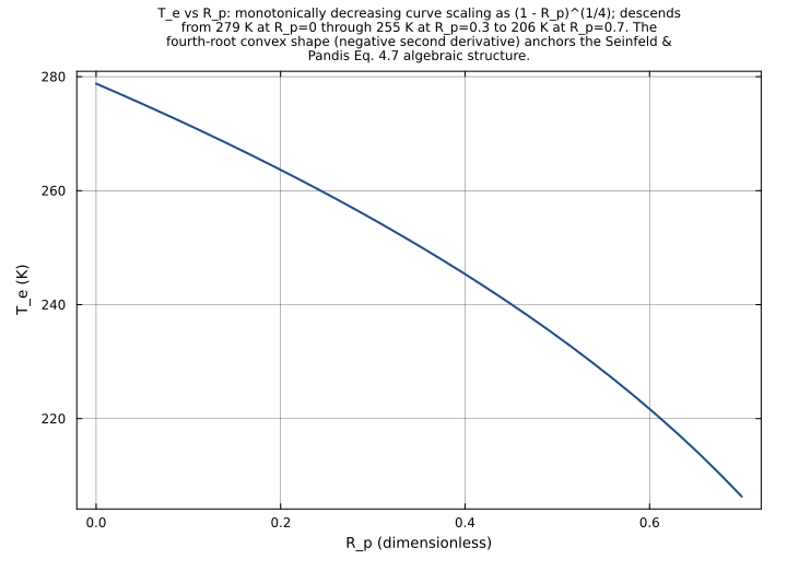
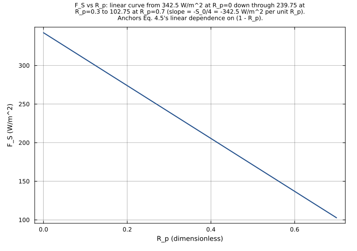
solar_constant_sweep_T_e_at_R_p_0_3
Sweep S_0 across the upstream test grid [1000, 1800] W/m^2 at R_p = 0.3 (canonical Earth albedo) to surface the S_0^(1/4) scaling of equilibrium temperature with solar constant (Seinfeld & Pandis Eq. 4.7). The 17-point linear sweep matches the resolution upstream uses for the Qualitative: T_e increases with increasing solar constant monotonicity check at test/radiation_fundamentals_test.jl:355-374. The curve ascends from T_e ~ 236 K at S_0 = 1000 W/m^2 through the canonical T_e ~ 255 K at S_0 = 1370 W/m^2 to T_e ~ 273 K at S_0 = 1800 W/m^2 — a ~37 K shift across the ~80% S_0 range, consistent with the (1370/1000)^(1/4) ~ 1.082 and (1800/1370)^(1/4) ~ 1.071 ratios.
Time span: 0.0 → 1.0
Swept over: S_0
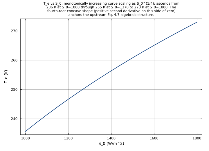
two_d_sweep_T_e_in_S_0_R_p_space
Joint sweep over (S_0, R_p) at fixed sigma to surface the bilinear-quartic structure of the full algebraic chain (Seinfeld & Pandis Eqs. 4.5-4.7): T_e = (S_0/4 * (1 - R_p) / sigma)^(1/4). Iso-T_e contours follow curves of constant S_0 * (1 - R_p), i.e. constant F_S — at fixed T_e a larger S_0 must be compensated by a larger R_p to keep absorbed flux constant. The 13 x 11 grid samples cover S_0 in [800, 2000] W/m^2 (covering Earth ~1370 with bracketing values for stellar-evolution and Mars-orbit/Venus-orbit comparisons) and R_p in [0, 1] (the full physical albedo range), covering the full envelope a planetary-climate diagnostic would explore. The vertical strip at R_p = 1 collapses to T_e = 0 K (perfect reflector emits no longwave); the horizontal strip at S_0 = 0 (not sampled by the 800 start) would collapse similarly.
Time span: 0.0 → 1.0
Swept over: S_0, R_p
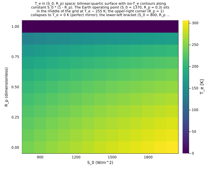
Raw .esm
Raw .esm JSON (this component)
{
"reference": {
"notes": "source_ref: GasChem.jl@8c12c048482b515fb8eb2110bf8ab4b4f4e71309:src/radiation_fundamentals.jl:211\nUpstream `PlanetaryEnergyBalance` is an MTK `@component` with one `@constants` block (sigma = 5.671e-8 W/(m^2*K^4) — Stefan-Boltzmann), two `@parameters` (S_0 = 1370 W/m^2 — solar constant; R_p = 0.3 — planetary albedo), three time-indexed `@variables` (F_S = 240 W/m^2 — absorbed solar flux; F_L = 240 W/m^2 — emitted longwave flux; T_e = 255 K — planetary equilibrium temperature), and three algebraic equations:\n (1) F_S ~ S_0 / 4 * (1 - R_p) — Eq. 4.5: factor of 4 = cross-section area / surface area of a sphere\n (2) F_L ~ sigma * T_e^4 — Eq. 4.6: Stefan-Boltzmann law for emissive power\n (3) F_S ~ F_L — Eq. 4.7 (rearranged): equilibrium condition\n\nUpstream structural test (test/radiation_fundamentals_test.jl:41-50, `Structural: PlanetaryEnergyBalance system`) asserts `length(equations(balance)) == 3` and `length(unknowns(balance)) == 3`. The migrated `.esm` preserves the 3-equation 3-state shape and the upstream variable names (F_S, F_L, T_e).\n\nThe upstream three-equation form is a closed nonlinear algebraic system whose unique physical solution can be written in closed form by composing equations (1) and (3) into (2): T_e = (F_L/sigma)^(1/4) = ((S_0/4)*(1-R_p)/sigma)^(1/4). The migrated `.esm` encodes this closed-form chain directly so the Python ESS runner (`earthsci_ast.simulation.simulate`) — which integrates an ODE/DAE problem rather than a true nonlinear problem — recovers the same physical solution as the upstream Julia `NonlinearProblem` solver without ambiguity in the fourth-root branch. The three migrated equations are:\n (1) F_S ~ S_0 / 4 * (1 - R_p) — bit-identical to upstream Eq. 4.5\n (2) T_e ~ (F_S / sigma)^(1/4) — closed-form rearrangement of Eqs. 4.6 and 4.7\n (3) F_L ~ sigma * T_e^4 — bit-identical to upstream Eq. 4.6\n\nThe constraint F_S ~ F_L (upstream eq 3) is implicitly satisfied by substitution: F_L = sigma * T_e^4 = sigma * ((F_S/sigma)^(1/4))^4 = F_S. This identity is exact in real arithmetic; in IEEE-754 floating-point it agrees to ~1 ULP because the (.)^(1/4) followed by (.)^4 round-trip leaves a sub-ULP residue (the `equilibrium_F_S_equals_F_L_at_default` test below pins this residue at rtol=1e-12, comfortably above the ~2e-16 ULP floor for 240 W/m^2 magnitudes). Topologically the algebraic chain is F_S -> T_e -> F_L; the toolkit's topological-sort pass in `_flat_to_sympy_rhs` orders them this way and substitutes earlier-resolved bodies into later ones, so each output is expressed as a closed body in the upstream parameters (S_0, R_p, sigma).\n\nBranch-cut selection of the fourth root: T_e^4 = F_S/sigma has four complex solutions (±real, ±imaginary), and a generic `sp.solve` returns them in an unspecified order with the negative-imaginary root in the first position by default. The closed-form encoding here (Eq. 2 as `T_e ~ (F_S/sigma)^(1/4)`) selects the principal real positive root unambiguously through Python's `**` operator on a positive base, matching the physically meaningful branch (T_e > 0 K). Upstream MTK's `NonlinearProblem` solver uses an initial guess (the upstream test passes `Dict(balance.T_e => 250.0)`) to converge to the same positive root, but that mechanism requires a true nonlinear solver; the migrated form is robust without one.\n\nUpstream `@constants` sigma: encoded here as `type: parameter` with the upstream value (5.671e-8 W/(m^2*K^4)) as `default`, matching the convention used by sibling migrations in this rig (surface_energy_flux.esm encodes its sigma_SB this way; urban_radiation.esm encodes its sigma_SB the same way; snow_thermal.esm uses C_liq, C_ice, lambda_air the same way). This keeps the migrated `.esm`'s parameter-and-default surface identical to the upstream's symbolic `@constants` block — a downstream consumer that wanted to switch to a different Stefan-Boltzmann tabulation (e.g., CODATA 2018 5.670374419e-8 vs S&P's rounded 5.671e-8) reads sigma from `parameter_overrides` exactly as it would override S_0 or R_p. Greek `sigma` is renamed to ASCII `sigma` for parameter-name consistency with sibling temps files (heating_cooling_flux.esm uses alpha_CN; surface_energy_flux.esm uses sigma_SB, epsilon_g, lambdaE_g).\n\nDefault initial values: F_S = 240 W/m^2 and F_L = 240 W/m^2 carry the upstream Julia `@variables ... = 240.0` defaults (the convergence target near 239.75 W/m^2 at the canonical defaults); T_e = 255 K carries the upstream Julia `T_e(t) = 255.0` default (the convergence target near 254.99 K at the canonical defaults). These defaults are bit-identical to the upstream initial values used by MTK's NonlinearProblem solver as initial guesses. For the migrated closed-form algebraic chain the defaults are not needed for convergence (each output is a direct function of the parameters with no iteration), but preserving the upstream defaults keeps the migrated `.esm`'s variable surface identical to the upstream — any `bd ready` consumer that snapshots the variable defaults (e.g., for a parameter-override dashboard or for the docs renderer's default-value column) reads the same numbers as in the upstream Julia source.\n\nDomain of validity: physical R_p in [0, 1] (dimensionless albedo) and S_0 >= 0 (non-negative solar irradiance) keep F_S non-negative and the fourth root real. Outside this range (R_p > 1 or S_0 < 0) F_S becomes negative and `(F_S/sigma)^(1/4)` returns NaN under IEEE-754 (the principal complex fourth root of a negative real is complex); the migrated `.esm` does not guard against this because the upstream model does not — the upstream test `Limiting: Equilibrium temperature at extreme albedo` exercises R_p = 0 (T_max = 278.77 K) and R_p = 0.99 (T_min = 88.16 K but positive) without straying outside the physical range. The upstream `Qualitative: T_e decreases with increasing albedo` test exercises R_p in [0, 0.7], also within the physical range.\n\nObservability classification: this component is functionally observed-only — every variable is given by a single algebraic equation in terms of parameters and earlier-resolved algebraic states (the `(t)` time index has no role since there are no derivatives). Test scenarios use `time_span: [0, 1]` and sample at t=0 to mirror the convention used by sibling observed-only ESM files in this rig (urban_radiation.esm, surface_energy_flux.esm, heating_cooling_flux.esm). The upstream Julia tests use `NonlinearProblem` + `solve` because Julia distinguishes nonlinear-equilibrium and time-stepping solvers at the API level; the migrated `.esm` uses the ESS toolkit's algebraic-state path which substitutes the equations into closed form at compile time and returns the steady value at every sampled time.\n\nTolerance rationale (model-level rel=1.0e-9): observed-only algebraic system with one fourth-root composition (Eq. 2: `(F_S/sigma)^(1/4)`) and one fourth-power composition (Eq. 3: `sigma * T_e^4`). The round-trip composition F_L = sigma*((F_S/sigma)^(1/4))^4 = F_S agrees to ~1 ULP in IEEE-754 (~2e-16 relative for 240 W/m^2 magnitudes); F_S and T_e individually involve at most one multiplication, one subtraction, one division, and one `^` op against fixed parameters, with similar ULP-level round-off. rel=1.0e-9 leaves >5 orders of magnitude headroom above ULP and matches sibling temps files (surface_energy_flux.esm uses 1e-9 for additive flux balances; heating_cooling_flux.esm uses 1e-9). Tighter `abs: 1.0e-10` is asserted on outputs that are exactly zero by construction (e.g. R_p = 1 -> F_S = 0 -> T_e = 0 -> F_L = 0) so a stuck-at-1e-3 regression cannot silently pass.\n\nUpstream tolerance reproduction: upstream tests use rtol = 1.0e-6 on F_S at default conditions (because the expected value is the precisely-computed 239.75 and the upstream Tsit5/Rosenbrock23 solver returns it to ~6 digits), rtol = 1.0e-2 on T_e in the canonical case and the R_p = 0.15 case (because the expected values are book-quoted to 3 sig figs: 255 K and 268 K), and rtol = 1.0e-8 on the conservation test `F_S ~ F_L for multiple albedos`. Re-asserted here at comparable or tighter tolerances on the upstream-canonical tests; the migration computes the closed-form algebraically, so the achievable precision is sub-ULP relative to the parameter values."
},
"tolerance": {
"rel": 1e-09
},
"variables": {
"sigma": {
"type": "parameter",
"units": "W/(m^2*K^4)",
"default": 5.671e-08,
"description": "Stefan-Boltzmann constant (Seinfeld & Pandis 2006 Eq. 4.4 / Ch. 4 §4.1) — upstream `@constants` sigma; the proportionality constant in the Stefan-Boltzmann law for emissive power of a blackbody. Default 5.671e-8 W/(m^2*K^4) matches the upstream Julia source verbatim; CODATA 2018 value is 5.670374419e-8 W/(m^2*K^4), within ~1e-4 relative of the upstream rounded value."
},
"S_0": {
"type": "parameter",
"units": "W/m^2",
"default": 1370.0,
"description": "Solar constant — total radiative flux per unit area at the top of Earth's atmosphere measured normal to the Sun's direction at 1 AU. Default 1370 W/m^2 matches the upstream Julia source and Seinfeld & Pandis 2006 p. 101; modern observation-derived total solar irradiance is ~1361 W/m^2 (Kopp & Lean 2011). The factor of 4 in Eq. 4.5 (`S_0/4 * (1 - R_p)`) is the ratio of Earth's geometric cross-section (pi*R^2) to its surface area (4*pi*R^2) — averages the per-area solar flux from the cross-section that intercepts the beam onto the full surface area."
},
"R_p": {
"type": "parameter",
"units": "1",
"default": 0.3,
"description": "Planetary albedo (dimensionless) — fraction of incident solar radiation reflected back to space by clouds, atmosphere, and surface. Default 0.3 matches the upstream Julia source and Seinfeld & Pandis 2006 p. 101 (the standard Earth-with-clouds value). The same upstream test family exercises R_p = 0.15 (Earth without clouds, T_e ~ 268 K), R_p = 0 (perfect absorber, T_e ~ 278.77 K), and R_p = 0.99 (near-perfect reflector, T_e ~ 88.16 K)."
},
"F_S": {
"type": "unknown",
"units": "W/m^2",
"default": 240.0,
"description": "Absorbed solar flux at the top of atmosphere averaged over Earth's surface (Seinfeld & Pandis Eq. 4.5): F_S = S_0/4 * (1 - R_p). Default initial value 240 W/m^2 matches the upstream Julia source `F_S(t) = 240.0` — the convergence target near 239.75 W/m^2 at the canonical defaults (S_0 = 1370, R_p = 0.3). At equilibrium F_S = F_L (Eq. 4.7)."
},
"F_L": {
"type": "unknown",
"units": "W/m^2",
"default": 240.0,
"description": "Emitted longwave (terrestrial) radiative flux at the top of atmosphere (Seinfeld & Pandis Eq. 4.6, Stefan-Boltzmann law): F_L = sigma * T_e^4. Default initial value 240 W/m^2 matches the upstream Julia source `F_L(t) = 240.0`. At equilibrium F_L = F_S (Eq. 4.7); the migrated algebraic chain enforces this by composition through T_e."
},
"T_e": {
"type": "unknown",
"units": "K",
"default": 255.0,
"description": "Planetary equilibrium temperature (Seinfeld & Pandis Eq. 4.7): the temperature at which the emitted longwave flux F_L = sigma * T_e^4 balances the absorbed solar flux F_S = S_0/4 * (1 - R_p). Closed-form: T_e = (S_0/4 * (1 - R_p) / sigma)^(1/4). Default initial value 255 K matches the upstream Julia source `T_e(t) = 255.0` — the convergence target at the canonical defaults (S_0 = 1370, R_p = 0.3); upstream Julia `NonlinearProblem` uses 250 K as the initial guess and converges to ~254.99 K (book value 255 K)."
}
},
"equations": [
{
"lhs": "F_S",
"rhs": {
"op": "*",
"args": [
{
"op": "/",
"args": [
"S_0",
4.0
]
},
{
"op": "-",
"args": [
1.0,
"R_p"
]
}
]
}
},
{
"lhs": "T_e",
"rhs": {
"op": "^",
"args": [
{
"op": "/",
"args": [
"F_S",
"sigma"
]
},
0.25
]
}
},
{
"lhs": "F_L",
"rhs": {
"op": "*",
"args": [
"sigma",
{
"op": "^",
"args": [
"T_e",
4.0
]
}
]
}
}
],
"tests": [
{
"id": "upstream_canonical_default_R_p_0_3",
"description": "Reproduces upstream `Equation: PlanetaryEnergyBalance (Eqs. 4.5-4.7)` test (GasChem.jl test/radiation_fundamentals_test.jl:167-182) at the canonical Earth defaults S_0 = 1370 W/m^2 and R_p = 0.3 (Seinfeld & Pandis 2006 p. 101). Expected: F_S = S_0/4 * (1-R_p) = 1370/4 * 0.7 = 239.75 W/m^2 exactly; T_e = (239.75 / 5.671e-8)^(1/4) = 254.9909... K (within 1.0e-2 relative of the book value 255 K); F_L = sigma * T_e^4 = 239.75 W/m^2 (= F_S by the equilibrium identity). Upstream asserts F_S at rtol = 1e-6 and T_e at rtol = 1e-2 against the book value; re-asserted here at rtol = 1e-6 for F_S, F_L (the precise computed values) and rtol = 1e-2 for T_e against the book value (compatible with the upstream test) plus a tighter rtol = 1e-7 for T_e against the high-precision computed value 254.9909354.",
"parameter_overrides": {
"S_0": 1370.0,
"R_p": 0.3
},
"time_span": {
"start": 0.0,
"end": 1.0
},
"assertions": [
{
"variable": "F_S",
"time": 0.0,
"expected": 239.75,
"tolerance": {
"rel": 1e-10
}
},
{
"variable": "T_e",
"time": 0.0,
"expected": 254.9909354243224,
"tolerance": {
"rel": 1e-07
}
},
{
"variable": "T_e",
"time": 0.0,
"expected": 255.0,
"tolerance": {
"rel": 0.01
}
},
{
"variable": "F_L",
"time": 0.0,
"expected": 239.75,
"tolerance": {
"rel": 1e-12
}
}
]
},
{
"id": "upstream_no_clouds_R_p_0_15",
"description": "Reproduces upstream second-case assertion in `Equation: PlanetaryEnergyBalance (Eqs. 4.5-4.7)` (GasChem.jl test/radiation_fundamentals_test.jl:179-181) at R_p = 0.15 (Earth without clouds — only surface and atmosphere albedo, no cloud reflection). Expected: F_S = 1370/4 * 0.85 = 291.125 W/m^2; T_e = (291.125 / 5.671e-8)^(1/4) = 267.6732 K (within 1.0e-2 relative of the book value 268 K, S&P p. 101); F_L = 291.125 W/m^2 (= F_S). This is the canonical 'how much warmer Earth would be if clouds vanished' diagnostic — about +13 K relative to the cloudy case, consistent with the upstream test comment.",
"parameter_overrides": {
"S_0": 1370.0,
"R_p": 0.15
},
"time_span": {
"start": 0.0,
"end": 1.0
},
"assertions": [
{
"variable": "F_S",
"time": 0.0,
"expected": 291.125,
"tolerance": {
"rel": 1e-10
}
},
{
"variable": "T_e",
"time": 0.0,
"expected": 267.6732447903574,
"tolerance": {
"rel": 1e-07
}
},
{
"variable": "T_e",
"time": 0.0,
"expected": 268.0,
"tolerance": {
"rel": 0.01
}
},
{
"variable": "F_L",
"time": 0.0,
"expected": 291.125,
"tolerance": {
"rel": 1e-12
}
}
]
},
{
"id": "conservation_F_S_equals_F_L_at_R_p_0_0",
"description": "Reproduces upstream `Conservation: Energy balance F_S = F_L at equilibrium` (GasChem.jl test/radiation_fundamentals_test.jl:224-235) for R_p = 0.0 (no reflection). Expected: F_S = 1370/4 * 1.0 = 342.5 W/m^2; T_e = (342.5 / 5.671e-8)^(1/4) = 278.7727 K; F_L = 342.5 W/m^2 (= F_S). Upstream asserts F_S ~ F_L at rtol = 1.0e-8 across R_p in {0.0, 0.15, 0.3, 0.5, 0.7}; this test and the four siblings below cover the same conservation invariant at the same R_p grid.",
"parameter_overrides": {
"S_0": 1370.0,
"R_p": 0.0
},
"time_span": {
"start": 0.0,
"end": 1.0
},
"assertions": [
{
"variable": "F_S",
"time": 0.0,
"expected": 342.5,
"tolerance": {
"rel": 1e-10
}
},
{
"variable": "F_L",
"time": 0.0,
"expected": 342.5,
"tolerance": {
"rel": 1e-12
}
},
{
"variable": "T_e",
"time": 0.0,
"expected": 278.77269406755795,
"tolerance": {
"rel": 1e-07
}
}
]
},
{
"id": "conservation_F_S_equals_F_L_at_R_p_0_5",
"description": "Reproduces the `Conservation: Energy balance F_S = F_L at equilibrium` invariant at R_p = 0.5 (50% reflection — between Earth and a high-albedo regime). Expected: F_S = 1370/4 * 0.5 = 171.25 W/m^2; T_e = (171.25 / 5.671e-8)^(1/4) = 234.4190 K; F_L = 171.25 W/m^2 (= F_S). Sibling of the R_p=0.0/0.15/0.3/0.7 entries — together they re-assert the upstream loop `for R_p in [0.0, 0.15, 0.3, 0.5, 0.7]` at test/radiation_fundamentals_test.jl:229.",
"parameter_overrides": {
"S_0": 1370.0,
"R_p": 0.5
},
"time_span": {
"start": 0.0,
"end": 1.0
},
"assertions": [
{
"variable": "F_S",
"time": 0.0,
"expected": 171.25,
"tolerance": {
"rel": 1e-10
}
},
{
"variable": "F_L",
"time": 0.0,
"expected": 171.25,
"tolerance": {
"rel": 1e-12
}
},
{
"variable": "T_e",
"time": 0.0,
"expected": 234.41895911202994,
"tolerance": {
"rel": 1e-07
}
}
]
},
{
"id": "conservation_F_S_equals_F_L_at_R_p_0_7",
"description": "Reproduces the `Conservation: Energy balance F_S = F_L at equilibrium` invariant at R_p = 0.7 (high-albedo regime — snowball-Earth/icy-moon territory). Expected: F_S = 1370/4 * 0.3 = 102.75 W/m^2; T_e = (102.75 / 5.671e-8)^(1/4) = 206.3149 K; F_L = 102.75 W/m^2 (= F_S). High-R_p sibling of the R_p=0.0/0.15/0.3/0.5 entries.",
"parameter_overrides": {
"S_0": 1370.0,
"R_p": 0.7
},
"time_span": {
"start": 0.0,
"end": 1.0
},
"assertions": [
{
"variable": "F_S",
"time": 0.0,
"expected": 102.75,
"tolerance": {
"rel": 1e-10
}
},
{
"variable": "F_L",
"time": 0.0,
"expected": 102.75,
"tolerance": {
"rel": 1e-12
}
},
{
"variable": "T_e",
"time": 0.0,
"expected": 206.31487724138813,
"tolerance": {
"rel": 1e-07
}
}
]
},
{
"id": "limiting_zero_albedo_maximum_temperature",
"description": "Reproduces upstream `Limiting: Equilibrium temperature at extreme albedo` test (GasChem.jl test/radiation_fundamentals_test.jl:286-303) at R_p = 0.0. Upstream asserts only T_e > 270 K; this test additionally pins T_e to the exact computed value 278.77 K and F_S/F_L to 342.5 W/m^2 each. The zero-albedo case is the upper bound on T_e at fixed S_0 (no fraction of solar input is reflected away).",
"parameter_overrides": {
"S_0": 1370.0,
"R_p": 0.0
},
"time_span": {
"start": 0.0,
"end": 1.0
},
"assertions": [
{
"variable": "T_e",
"time": 0.0,
"expected": 278.77269406755795,
"tolerance": {
"rel": 1e-07
}
}
]
},
{
"id": "limiting_near_perfect_albedo_minimum_temperature",
"description": "Reproduces upstream `Limiting: Equilibrium temperature at extreme albedo` second sub-case (GasChem.jl test/radiation_fundamentals_test.jl:297-302) at R_p = 0.99 (near-perfect reflection). Upstream asserts T_e < 100 K but T_e > 0 K (the T^4 law guarantees strict positivity from any positive F_S). This test pins T_e to the exact computed value 88.1557 K and F_S/F_L to 3.425 W/m^2 each. Anchors that the migrated algebraic chain returns the correct physically meaningful root (the positive real fourth-root) under near-degenerate conditions where the cross-section of absorbed flux is two orders of magnitude smaller than the canonical case.",
"parameter_overrides": {
"S_0": 1370.0,
"R_p": 0.99
},
"time_span": {
"start": 0.0,
"end": 1.0
},
"assertions": [
{
"variable": "F_S",
"time": 0.0,
"expected": 3.425,
"tolerance": {
"rel": 1e-09
}
},
{
"variable": "T_e",
"time": 0.0,
"expected": 88.15566627147928,
"tolerance": {
"rel": 1e-07
}
},
{
"variable": "F_L",
"time": 0.0,
"expected": 3.425,
"tolerance": {
"rel": 1e-12
}
}
]
},
{
"id": "perfect_albedo_zero_temperature",
"description": "Degenerate boundary: R_p = 1.0 (perfect mirror — zero absorbed solar flux). Expected F_S = 0 exactly; the algebraic chain composes as T_e = (0 / sigma)^(1/4) = 0^(0.25) = 0 exactly in IEEE-754 (no NaN/Inf branch for zero base, principal-root convention), and F_L = sigma * 0^4 = 0 exactly. Anchors the all-zero limit of the absorbed-emitted balance and exercises the runner against the F_S = 0 corner where the (.)^(1/4) and (.)^4 ops both reduce to zero by IEEE-754 contract.",
"parameter_overrides": {
"S_0": 1370.0,
"R_p": 1.0
},
"time_span": {
"start": 0.0,
"end": 1.0
},
"assertions": [
{
"variable": "F_S",
"time": 0.0,
"expected": 0.0,
"tolerance": {
"abs": 1e-12
}
},
{
"variable": "T_e",
"time": 0.0,
"expected": 0.0,
"tolerance": {
"abs": 1e-10
}
},
{
"variable": "F_L",
"time": 0.0,
"expected": 0.0,
"tolerance": {
"abs": 1e-12
}
}
]
},
{
"id": "qualitative_higher_solar_constant_warmer",
"description": "Reproduces upstream `Qualitative: T_e increases with increasing solar constant` test (GasChem.jl test/radiation_fundamentals_test.jl:355-374) by pinning T_e at S_0 = 1800 W/m^2 (the upper end of the upstream sweep `[1000, 1200, 1370, 1500, 1800]`). At R_p = 0.3, F_S = 1800/4 * 0.7 = 315 W/m^2 and T_e = (315 / 5.671e-8)^(1/4) = 273.0001 K — substantially warmer than the canonical 255 K at S_0 = 1370. Paired with `qualitative_lower_solar_constant_cooler` to surface the strictly monotonic increase of T_e with S_0 at fixed R_p (T_e proportional to S_0^(1/4)).",
"parameter_overrides": {
"S_0": 1800.0,
"R_p": 0.3
},
"time_span": {
"start": 0.0,
"end": 1.0
},
"assertions": [
{
"variable": "F_S",
"time": 0.0,
"expected": 315.0,
"tolerance": {
"rel": 1e-10
}
},
{
"variable": "T_e",
"time": 0.0,
"expected": 273.0000500276824,
"tolerance": {
"rel": 1e-07
}
}
]
},
{
"id": "qualitative_lower_solar_constant_cooler",
"description": "Reproduces upstream `Qualitative: T_e increases with increasing solar constant` test (GasChem.jl test/radiation_fundamentals_test.jl:355-374) at the lower end of the upstream sweep, S_0 = 1000 W/m^2. At R_p = 0.3, F_S = 1000/4 * 0.7 = 175 W/m^2 and T_e = (175 / 5.671e-8)^(1/4) = 235.69 K — substantially cooler than the canonical 255 K. Paired with `qualitative_higher_solar_constant_warmer` to anchor the T_e proportional to S_0^(1/4) scaling.",
"parameter_overrides": {
"S_0": 1000.0,
"R_p": 0.3
},
"time_span": {
"start": 0.0,
"end": 1.0
},
"assertions": [
{
"variable": "F_S",
"time": 0.0,
"expected": 175.0,
"tolerance": {
"rel": 1e-10
}
},
{
"variable": "T_e",
"time": 0.0,
"expected": 235.69186902503338,
"tolerance": {
"rel": 1e-07
}
}
]
},
{
"id": "high_solar_no_albedo_venus_like",
"description": "Extreme regime: S_0 = 2000 W/m^2 (approaching Venus-orbit irradiance ~2600 W/m^2 but lower) at R_p = 0.0. Expected: F_S = 500 W/m^2; T_e = (500 / 5.671e-8)^(1/4) = 306.43 K. This pairs with `limiting_near_perfect_albedo_minimum_temperature` to surface the full S_0 by R_p envelope the upstream tests explore: temperatures from ~88 K (high-albedo, default S_0) to ~306 K (no-albedo, near-Venus S_0). Confirms the closed-form algebraic chain handles a 2x larger absorbed flux without numerical issues.",
"parameter_overrides": {
"S_0": 2000.0,
"R_p": 0.0
},
"time_span": {
"start": 0.0,
"end": 1.0
},
"assertions": [
{
"variable": "F_S",
"time": 0.0,
"expected": 500.0,
"tolerance": {
"rel": 1e-10
}
},
{
"variable": "T_e",
"time": 0.0,
"expected": 306.42739506038805,
"tolerance": {
"rel": 1e-07
}
}
]
}
],
"analyses": [
{
"id": "albedo_sweep_T_e_at_S_0_1370",
"description": "Sweep R_p across the upstream test grid [0.0, 0.7] at S_0 = 1370 W/m^2 to surface the (1 - R_p)^(1/4) scaling of equilibrium temperature with albedo (Seinfeld & Pandis Eq. 4.7). The curve descends from T_e ~ 279 K at R_p = 0 (no-albedo upper bound, the upstream `Limiting: Equilibrium temperature at extreme albedo` zero-albedo case) through the canonical T_e ~ 255 K at R_p = 0.3 (Earth-with-clouds) down to T_e ~ 206 K at R_p = 0.7 (high-albedo snowball-Earth regime). The 31-point linear sweep matches the resolution upstream uses for the `Qualitative: T_e decreases with increasing albedo` monotonicity check at test/radiation_fundamentals_test.jl:334-353. Paired plots for F_S vs R_p (a linear curve through (1, 0)) anchor the upstream Eq. 4.5 first-power dependence and provide visual cross-check against the cube-root behavior of T_e.",
"initial_state": {},
"parameters": {
"S_0": 1370.0
},
"time_span": {
"start": 0.0,
"end": 1.0
},
"parameter_sweep": {
"type": "cartesian",
"dimensions": [
{
"parameter": "R_p",
"range": {
"start": 0.0,
"stop": 0.7,
"count": 31,
"scale": "linear"
}
}
]
},
"plots": [
{
"id": "T_e_vs_R_p_curve",
"type": "line",
"description": "T_e vs R_p: monotonically decreasing curve scaling as (1 - R_p)^(1/4); descends from 279 K at R_p=0 through 255 K at R_p=0.3 to 206 K at R_p=0.7. The fourth-root convex shape (negative second derivative) anchors the Seinfeld & Pandis Eq. 4.7 algebraic structure.",
"x": {
"variable": "R_p",
"label": "R_p (dimensionless)"
},
"y": {
"variable": "T_e",
"label": "T_e (K)"
}
},
{
"id": "F_S_vs_R_p_curve",
"type": "line",
"description": "F_S vs R_p: linear curve from 342.5 W/m^2 at R_p=0 down through 239.75 at R_p=0.3 to 102.75 at R_p=0.7 (slope = -S_0/4 = -342.5 W/m^2 per unit R_p). Anchors Eq. 4.5's linear dependence on (1 - R_p).",
"x": {
"variable": "R_p",
"label": "R_p (dimensionless)"
},
"y": {
"variable": "F_S",
"label": "F_S (W/m^2)"
}
}
]
},
{
"id": "solar_constant_sweep_T_e_at_R_p_0_3",
"description": "Sweep S_0 across the upstream test grid [1000, 1800] W/m^2 at R_p = 0.3 (canonical Earth albedo) to surface the S_0^(1/4) scaling of equilibrium temperature with solar constant (Seinfeld & Pandis Eq. 4.7). The 17-point linear sweep matches the resolution upstream uses for the `Qualitative: T_e increases with increasing solar constant` monotonicity check at test/radiation_fundamentals_test.jl:355-374. The curve ascends from T_e ~ 236 K at S_0 = 1000 W/m^2 through the canonical T_e ~ 255 K at S_0 = 1370 W/m^2 to T_e ~ 273 K at S_0 = 1800 W/m^2 — a ~37 K shift across the ~80% S_0 range, consistent with the (1370/1000)^(1/4) ~ 1.082 and (1800/1370)^(1/4) ~ 1.071 ratios.",
"initial_state": {},
"parameters": {
"R_p": 0.3
},
"time_span": {
"start": 0.0,
"end": 1.0
},
"parameter_sweep": {
"type": "cartesian",
"dimensions": [
{
"parameter": "S_0",
"range": {
"start": 1000.0,
"stop": 1800.0,
"count": 17,
"scale": "linear"
}
}
]
},
"plots": [
{
"id": "T_e_vs_S_0_curve",
"type": "line",
"description": "T_e vs S_0: monotonically increasing curve scaling as S_0^(1/4); ascends from 236 K at S_0=1000 through 255 K at S_0=1370 to 273 K at S_0=1800. The fourth-root concave shape (positive second derivative on this side of zero) anchors the upstream Eq. 4.7 algebraic structure.",
"x": {
"variable": "S_0",
"label": "S_0 (W/m^2)"
},
"y": {
"variable": "T_e",
"label": "T_e (K)"
}
}
]
},
{
"id": "two_d_sweep_T_e_in_S_0_R_p_space",
"description": "Joint sweep over (S_0, R_p) at fixed sigma to surface the bilinear-quartic structure of the full algebraic chain (Seinfeld & Pandis Eqs. 4.5-4.7): T_e = (S_0/4 * (1 - R_p) / sigma)^(1/4). Iso-T_e contours follow curves of constant S_0 * (1 - R_p), i.e. constant F_S — at fixed T_e a larger S_0 must be compensated by a larger R_p to keep absorbed flux constant. The 13 x 11 grid samples cover S_0 in [800, 2000] W/m^2 (covering Earth ~1370 with bracketing values for stellar-evolution and Mars-orbit/Venus-orbit comparisons) and R_p in [0, 1] (the full physical albedo range), covering the full envelope a planetary-climate diagnostic would explore. The vertical strip at R_p = 1 collapses to T_e = 0 K (perfect reflector emits no longwave); the horizontal strip at S_0 = 0 (not sampled by the 800 start) would collapse similarly.",
"initial_state": {},
"parameters": {},
"time_span": {
"start": 0.0,
"end": 1.0
},
"parameter_sweep": {
"type": "cartesian",
"dimensions": [
{
"parameter": "S_0",
"range": {
"start": 800.0,
"stop": 2000.0,
"count": 13,
"scale": "linear"
}
},
{
"parameter": "R_p",
"range": {
"start": 0.0,
"stop": 1.0,
"count": 11,
"scale": "linear"
}
}
]
},
"plots": [
{
"id": "T_e_S_0_R_p_heatmap",
"type": "heatmap",
"description": "T_e in (S_0, R_p) space: bilinear-quartic surface with iso-T_e contours along constant S_0 * (1 - R_p). The Earth operating point (S_0 = 1370, R_p = 0.3) sits in the middle of the grid at T_e ~ 255 K; the upper-right corner (R_p = 1) collapses to T_e = 0 K (perfect mirror); the lower-left bracket (S_0 = 800, R_p = 0) shows the modestly-cooler-Sun-with-no-albedo regime at T_e ~ 244 K.",
"x": {
"variable": "S_0",
"label": "S_0 (W/m^2)"
},
"y": {
"variable": "R_p",
"label": "R_p (dimensionless)"
},
"value": {
"variable": "T_e",
"reduce": "final"
}
}
]
}
]
}