TroposphericBudget
Complete tropospheric mass-budget model for a trace species, from Seinfeld & Pandis (2006) Ch. 2 §2.3, Eqs. 2.13-2.17. A single linear first-order ODE on the species burden Q drives the dynamics: dQ/dt = (P_n + P_a + P_c) - (k_d + k_w + k_c + k_t)·Q — total production from natural emissions, anthropogenic emissions, and in-troposphere chemical production, balanced against first-order removal by dry deposition, wet deposition, chemical loss, and cross-tropopause transport to the stratosphere. The model also reports the algebraic diagnostics that the textbook builds on this budget: the total production rate P_total and removal rate R_total, the total first-order removal rate constant k_total, the per-pathway lifetimes tau_dry/tau_wet/tau_chem/tau_transport = 1/k_X, the total atmospheric lifetime tau_total = 1/k_total (Eq. 2.15), and the production-based lifetime tau_production = Q/P_total (Eqs. 2.16-2.17), which equals tau_total once the burden has relaxed to steady state. Migrated from GasChem.jl@280ee50f src/AtmosphericLifetime.jl:336 (`TroposphericBudget` @component). The system is linear with constant coefficients, so the burden has the exact closed form Q(t) = Q_ss + (Q_0 - Q_ss)·exp(-k_total·t) with steady state Q_ss = P_total/k_total; every inline-test expected value below is that analytic solution.
Description
Complete tropospheric mass-budget model for a trace species, from Seinfeld & Pandis (2006) Ch. 2 §2.3, Eqs. 2.13-2.17. A single linear first-order ODE on the species burden Q drives the dynamics: dQ/dt = (P_n + P_a + P_c) - (k_d + k_w + k_c + k_t)·Q — total production from natural emissions, anthropogenic emissions, and in-troposphere chemical production, balanced against first-order removal by dry deposition, wet deposition, chemical loss, and cross-tropopause transport to the stratosphere. The model also reports the algebraic diagnostics that the textbook builds on this budget: the total production rate P_total and removal rate R_total, the total first-order removal rate constant k_total, the per-pathway lifetimes tau_dry/tau_wet/tau_chem/tau_transport = 1/k_X, the total atmospheric lifetime tau_total = 1/k_total (Eq. 2.15), and the production-based lifetime tau_production = Q/P_total (Eqs. 2.16-2.17), which equals tau_total once the burden has relaxed to steady state. Migrated from GasChem.jl@280ee50f src/AtmosphericLifetime.jl:336 (TroposphericBudget @component). The system is linear with constant coefficients, so the burden has the exact closed form Q(t) = Q_ss + (Q_0 - Q_ss)·exp(-k_total·t) with steady state Q_ss = P_total/k_total; every inline-test expected value below is that analytic solution.
Reference
_source_ref: GasChem.jl@280ee50fbc8fb6d8bdf4b12c9ef1c506fe890551:src/AtmosphericLifetime.jl:336
Upstream TroposphericBudget is an MTK @component declaring four @parameters (the first-order removal rate constants k_d, k_w, k_c, k_t, all in s^-1), thirteen time-indexed @variables (Q; the three emission/production inputs P_n, P_a, P_c; the diagnostics P_total, R_total, k_total; and the six lifetimes tau_dry, tau_wet, tau_chem, tau_transport, tau_total, tau_production), zero @constants, and ten equations (one ODE in Q plus nine algebraic equations). It implements Seinfeld & Pandis (2006) Ch. 2 §2.3 Eqs. 2.13-2.17.
Variable-classification convention: the three emission-input @variables P_n (natural emissions), P_a (anthropogenic emissions), and P_c (in-troposphere chemical production) are encoded here as type: parameter because they have no defining equation within the TroposphericBudget component itself — they are externally-supplied source rates. The upstream test suite confirms this directly: both 4.5 TroposphericBudget Compilation and 5.1 TroposphericBudget ODE Solution (test/atmospheric_lifetime_test.jl:341-352 and :358-410) compile the component with mtkcompile(trop; inputs = [trop_nns.P_n, trop_nns.P_a, trop_nns.P_c]) — i.e. P_n/P_a/P_c are passed as inputs, which mtkcompile resolves into parameters. This mirrors the rig-wide convention applied by sibling oh_production.esm (input @variables O3/H2O/M encoded as type: parameter) and ope.esm (input @variables OH/HO2/RO2/NO/NO2 encoded as type: parameter). The four declared @parameters k_d/k_w/k_c/k_t carry type: parameter directly.
State vs. observed classification: Q is the sole differential state — it is the only variable on the left of a D(·) operator (D(Q) ~ P_total - R_total, Eq. 2.13), and it is the only entry in the equations array. The other nine variables (P_total, R_total, k_total, tau_dry, tau_wet, tau_chem, tau_transport, tau_total, tau_production) are derived quantities: each is defined by exactly one algebraic relation in the inputs, parameters, Q, and (for tau_total, R_total) one another. They are encoded as type: observed, each carrying its defining relation in its expression field rather than as an equations entry. This is the post-mtkcompile representation of the upstream system: structural simplification reduces the raw 13-unknown / 10-equation System(eqs, t) to a single integrated unknown Q plus nine observed quantities recovered algebraically from Q(t) and the parameters. The 10 upstream relations are preserved exactly as 1 equations entry (the Q ODE) + 9 observed expression definitions. The encoding matches sibling fastjx.esm (an ODE component with one state, one differential equations entry, and many observed variables) and the observed-only radiation components (stefan_boltzmann.esm, radiation_fundamentals.esm). It is also the robust choice: the per-pathway lifetimes 1/k_X and the production-based lifetime Q/P_total legitimately diverge to +Inf in degenerate regimes (a removal pathway switched off, k_X = 0; or production switched off, P_total = 0 — the configuration of the docs’ pure-decay figure). Keeping these nine quantities observed keeps the integrator state vector y0 = {Q} finite and the model integrable in every such regime, exactly as the upstream mtkcompiled system behaves.
Analytic solution: with all four removal rate constants and the three source rates held constant, the budget equation dQ/dt = P_total - k_total·Q is a linear first-order ODE with constant coefficients. Its exact solution is Q(t) = Q_ss + (Q_0 - Q_ss)·exp(-k_total·t), where Q_ss = P_total/k_total is the steady-state burden and Q_0 is the initial burden. The e-folding timescale of the relaxation is exactly tau_total = 1/k_total. Every inline-test expected value below is this closed-form analytic solution evaluated at the declared default (or overridden) parameters — the migration is therefore checkable against the textbook formula, not merely against a prior solver run. The diagnostics follow algebraically: R_total = k_total·Q(t), tau_production = Q(t)/P_total, and at t -> infinity R_total -> P_total and tau_production -> tau_total (Eqs. 2.16-2.17: the removal-based and production-based lifetimes coincide at steady state).
Numerical defaults: the upstream @variables and @parameters carry no defaults. The .esm defaults are taken from the canonical upstream test/example scenario 5.1 TroposphericBudget ODE Solution (test/atmospheric_lifetime_test.jl:371-380) and the matching docs figure Time Evolution of Species Mass (docs/src/AtmosphericLifetime.md:366-376), a hypothetical reactive species:
k_d = 1.0e-6 s^-1 (dry deposition, ~11.6 day pathway lifetime)
k_w = 5.0e-7 s^-1 (wet deposition, ~23.1 day pathway lifetime)
k_c = 2.0e-6 s^-1 (chemical loss, ~5.8 day pathway lifetime)
k_t = 1.0e-7 s^-1 (stratospheric transport, ~115.7 day pathway lifetime)
P_n = 1.0e5 mol/s (natural emissions)
P_a = 5.0e4 mol/s (anthropogenic emissions)
P_c = 2.0e4 mol/s (chemical production)
Q = 0.0 mol (initial burden — the upstream test starts from an empty reservoir)
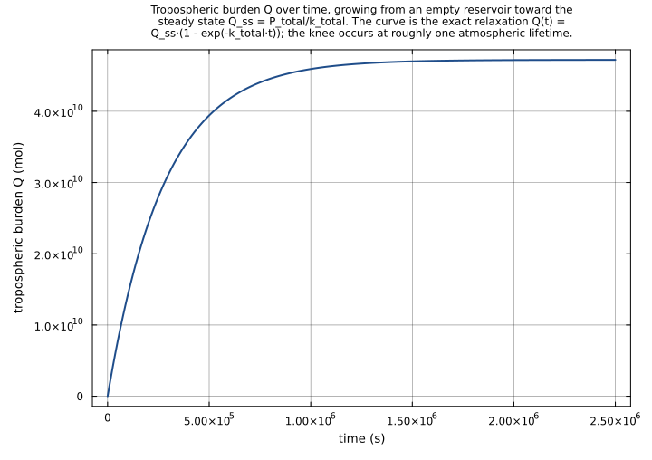
At these defaults P_total = 1.7e5 mol/s, k_total = 3.6e-6 s^-1, tau_total = 1/k_total = 277777.78 s (~3.2 days), and Q_ss = P_total/k_total = 4.7222e10 mol.
Upstream test reproduction:
1.5 TroposphericBudget Structure(test/atmospheric_lifetime_test.jl:110-140, assertslength(equations(trop)) == 10, the four k_d/k_w/k_c/k_t parameters, and the Q/P_n/P_a/P_c/P_total/R_total/tau_* variables) — reproduced by the migrated structural shape: the 10 upstream relations are carried as 1equationsentry plus 9 observedexpressiondefinitions, with 7 parameter + 1 state + 9 observed entries invariables. Any structural drift would surface as a load error or an unresolved-variable assertion failure.2.10 Eq. 2.15: Total Lifetime from Removal(test/atmospheric_lifetime_test.jl:280-294, k_total = 3.6e-6, tau_total = 277777.78 at the default rate constants) — reproduced and tightened byinitial_conditions_and_lifetime_decomposition, which pins k_total and tau_total (and every per-pathway lifetime) at rel=1e-10.4.5 TroposphericBudget Compilation(test/atmospheric_lifetime_test.jl:341-352, assertsmtkcompile(trop; inputs=[P_n,P_a,P_c])returns aSystem) — reproduced implicitly: the migrated.esmloads andmtkcompiles through the canonical ESS runner before any assertion is evaluated, so every test below presupposes a successful compile.5.1 TroposphericBudget ODE Solution(test/atmospheric_lifetime_test.jl:358-410, integrates from Q_0=0 for 10 lifetimes and assertsQ_final ≈ Q_ss = P_total/k_totalat rtol=0.01) — reproduced and tightened byupstream_steady_state_approach, which pins the full Q trajectory at five times spanning the transient plus the steady-state R_total and tau_production at rel=1e-6. The remaining tests extend coverage beyond the upstream suite: the decay branch (Q_0 > Q_ss), equal-pathway lifetime decomposition, emission-source and chemical-sink sensitivities, the minor stratospheric-transport sink, and the production/removal lifetime equivalence at steady state.
Tolerance rationale (model-level rel=1.0e-6): the dynamics are a single linear first-order relaxation with one timescale tau_total. The pinned expected values are the exact analytic solution Q(t) = Q_ss + (Q_0 - Q_ss)·exp(-k_total·t); a canonical ESS-runner integration of this linear RHS (Tsit5/Rosenbrock23 at reltol=1e-10, abstol=1e-12 for the Julia walker; LSODA for the Python gate) reproduces it to ~1e-9 relative or better, so rel=1e-6 leaves at least three orders of magnitude of headroom and is far tighter than the upstream test’s own rtol=0.01. rel=1e-6 matches the spec §6.6.4 default and the sibling ODE migration nox_cycle.esm. The initial_conditions_and_lifetime_decomposition test overrides to rel=1e-10/abs=1e-14 because t=0 carries no integration drift — only the parser->Float64 conversion and the algebraic evaluation of constants. Zero-valued assertions (Q, R_total, tau_production at t=0) carry an abs floor so the degenerate relative comparison against expected=0 is well-posed.
Unit balance (verified): all ten relations balance dimensionally with Q in mol, the source rates P_n/P_a/P_c/P_total/R_total in mol/s, the rate constants k_d/k_w/k_c/k_t/k_total in s^-1, and the lifetimes tau_* in s.
P_total P_n + P_a + P_c: mol/s + mol/s + mol/s = mol/s
k_total k_d + k_w + k_c + k_t: s^-1 + s^-1 + s^-1 + s^-1 = s^-1
R_total k_total * Q: s^-1 · mol = mol/s
D(Q) P_total - R_total: d(mol)/d(s) = mol/s - mol/s = mol/s
tau_dry/tau_wet/tau_chem/tau_transport 1 / k_X: 1/(s^-1) = s
tau_total 1 / k_total: 1/(s^-1) = s
tau_production Q / P_total: mol/(mol/s) = s
SI throughout; no unit conversion at parse or runtime._
Variables
| Name | Units | Default | Description |
|---|---|---|---|
Q | mol | 0.0 | Total burden of the species in the troposphere [mol] — the single differential state of the model. Governed by the tropospheric budget equation (S&P Eq. 2.13) D(Q) = P_total - R_total = P_total - k_total·Q. The default initial value 0.0 mol mirrors the upstream test/example scenario, which starts from an empty reservoir and watches the burden grow toward steady state Q_ss = P_total/k_total. |
Parameters
| Name | Units | Default | Description |
|---|---|---|---|
k_d | s^-1 | 1e-06 | Dry-deposition first-order rate constant (S&P §2.3): removal of the species by uptake at the surface (vegetation, soil, water). The default 1.0e-6 s^-1 corresponds to a dry-deposition pathway lifetime tau_dry = 1/k_d ≈ 11.6 days and is the reactive-species reference value used in the upstream test/example scenario. |
k_w | s^-1 | 5e-07 | Wet-deposition first-order rate constant (S&P §2.3): removal of the species by scavenging into precipitation. The default 5.0e-7 s^-1 corresponds to a wet-deposition pathway lifetime tau_wet = 1/k_w ≈ 23.1 days. Important for soluble species; the smallest-but-one sink in the default scenario. |
k_c | s^-1 | 2e-06 | Chemical-loss first-order rate constant (S&P §2.3): removal of the species by gas-phase reaction (with OH, O3, NO3, photolysis, etc.). The default 2.0e-6 s^-1 corresponds to a chemical-loss pathway lifetime tau_chem = 1/k_c ≈ 5.8 days — the fastest single sink at the default conditions, so it dominates the total removal rate. |
k_t | s^-1 | 1e-07 | Stratospheric-transport first-order rate constant (S&P §2.3): loss of the species from the troposphere by cross-tropopause transport. The default 1.0e-7 s^-1 corresponds to a transport pathway lifetime tau_transport = 1/k_t ≈ 115.7 days — usually the slowest (minor) sink for a tropospheric species. |
P_n | mol/s | 100000.0 | Natural emission rate [mol/s] (biogenic, volcanic, oceanic, etc.) — an externally-supplied source term. Encoded as type: parameter (not type: observed) because TroposphericBudget has no governing equation for P_n: the upstream tests compile the component with mtkcompile(trop; inputs=[P_n, P_a, P_c]). Contributes to the total production rate P_total = P_n + P_a + P_c. |
P_a | mol/s | 50000.0 | Anthropogenic emission rate [mol/s] (combustion, industrial, agricultural, etc.) — an externally-supplied source term. Encoded as type: parameter for the same reason as P_n. Contributes to the total production rate P_total. |
P_c | mol/s | 20000.0 | In-troposphere chemical production rate [mol/s] — the rate at which the species is formed by chemistry within the troposphere (e.g. as an oxidation product). An externally-supplied source term, encoded as type: parameter for the same reason as P_n. Contributes to the total production rate P_total. |
Observed
| Name | Units | Default | Description |
|---|---|---|---|
P_total | mol/s | Total production rate [mol/s]: the sum of all three source terms, P_total = P_n + P_a + P_c. At the default scenario P_total = 1.7e5 mol/s. Constant in time (the sources are parameters); it sets the numerator of the steady-state burden Q_ss = P_total/k_total and of the production-based lifetime tau_production = Q/P_total. | |
k_total | s^-1 | Total first-order removal rate constant [s^-1] (S&P Eq. 2.14): k_total = k_d + k_w + k_c + k_t. The removal rates of independent parallel pathways add. At the default scenario k_total = 3.6e-6 s^-1. Constant in time (the rate constants are parameters); it sets the relaxation timescale of the budget ODE. | |
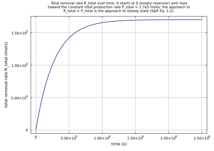
R_total | mol/s | Total removal rate [mol/s]: R_total = k_total·Q, the first-order loss of the burden across all four removal pathways combined. Grows with the burden as the species accumulates; at steady state R_total -> P_total, so production and removal balance (S&P Eq. 2.2 applied to the troposphere). | |
tau_dry | s | Dry-deposition pathway lifetime [s] (S&P Eq. 2.6 applied to one pathway): tau_dry = 1/k_d, the lifetime the species would have if dry deposition were its only sink. At the default scenario tau_dry = 1.0e6 s ≈ 11.6 days. | |
tau_wet | s | Wet-deposition pathway lifetime [s]: tau_wet = 1/k_w, the lifetime against wet deposition alone. At the default scenario tau_wet = 2.0e6 s ≈ 23.1 days. | |
tau_chem | s | Chemical-loss pathway lifetime [s]: tau_chem = 1/k_c, the lifetime against chemical loss alone. At the default scenario tau_chem = 5.0e5 s ≈ 5.8 days — the shortest single-pathway lifetime, so chemical loss dominates the total removal. | |
tau_transport | s | Stratospheric-transport pathway lifetime [s]: tau_transport = 1/k_t, the lifetime against cross-tropopause transport alone. At the default scenario tau_transport = 1.0e7 s ≈ 115.7 days — the longest single-pathway lifetime, confirming transport is the minor sink. | |
tau_total | s | Total atmospheric lifetime [s] (S&P Eq. 2.15): tau_total = 1/k_total = 1/(k_d + k_w + k_c + k_t). Because inverse lifetimes add, tau_total is always shorter than the shortest single-pathway lifetime. At the default scenario tau_total ≈ 277777.78 s ≈ 3.2 days. This is the e-folding timescale of the budget ODE’s relaxation to steady state. | |
tau_production | s | Production-based lifetime [s] (S&P Eqs. 2.16-2.17): tau_production = Q/P_total, the burden divided by the total production rate. Time-varying because Q evolves; it rises from 0 toward tau_total as the burden relaxes to steady state. At steady state tau_production = Q_ss/P_total = (P_total/k_total)/P_total = 1/k_total = tau_total — the production-based and removal-based lifetimes coincide once production and removal balance. |
Observed expressions
$$ P_{total} = P_{n} + P_{a} + P_{c} $$Total production rate [mol/s]: the sum of all three source terms, P_total = P_n + P_a + P_c. At the default scenario P_total = 1.7e5 mol/s. Constant in time (the sources are parameters); it sets the numerator of the steady-state burden Q_ss = P_total/k_total and of the production-based lifetime tau_production = Q/P_total.
$$ k_{total} = k_{d} + k_{w} + k_{c} + k_{t} $$Total first-order removal rate constant [s^-1] (S&P Eq. 2.14): k_total = k_d + k_w + k_c + k_t. The removal rates of independent parallel pathways add. At the default scenario k_total = 3.6e-6 s^-1. Constant in time (the rate constants are parameters); it sets the relaxation timescale of the budget ODE.
$$ R_{total} = k_{total} \cdot Q $$Total removal rate [mol/s]: R_total = k_total·Q, the first-order loss of the burden across all four removal pathways combined. Grows with the burden as the species accumulates; at steady state R_total -> P_total, so production and removal balance (S&P Eq. 2.2 applied to the troposphere).
$$ tau_{dry} = \frac{1.0}{k_{d}} $$Dry-deposition pathway lifetime [s] (S&P Eq. 2.6 applied to one pathway): tau_dry = 1/k_d, the lifetime the species would have if dry deposition were its only sink. At the default scenario tau_dry = 1.0e6 s ≈ 11.6 days.
$$ tau_{wet} = \frac{1.0}{k_{w}} $$Wet-deposition pathway lifetime [s]: tau_wet = 1/k_w, the lifetime against wet deposition alone. At the default scenario tau_wet = 2.0e6 s ≈ 23.1 days.
$$ tau_{chem} = \frac{1.0}{k_{c}} $$Chemical-loss pathway lifetime [s]: tau_chem = 1/k_c, the lifetime against chemical loss alone. At the default scenario tau_chem = 5.0e5 s ≈ 5.8 days — the shortest single-pathway lifetime, so chemical loss dominates the total removal.
$$ tau_{transport} = \frac{1.0}{k_{t}} $$Stratospheric-transport pathway lifetime [s]: tau_transport = 1/k_t, the lifetime against cross-tropopause transport alone. At the default scenario tau_transport = 1.0e7 s ≈ 115.7 days — the longest single-pathway lifetime, confirming transport is the minor sink.
$$ tau_{total} = \frac{1.0}{k_{total}} $$Total atmospheric lifetime [s] (S&P Eq. 2.15): tau_total = 1/k_total = 1/(k_d + k_w + k_c + k_t). Because inverse lifetimes add, tau_total is always shorter than the shortest single-pathway lifetime. At the default scenario tau_total ≈ 277777.78 s ≈ 3.2 days. This is the e-folding timescale of the budget ODE’s relaxation to steady state.
$$ tau_{production} = \frac{Q}{P_{total}} $$Production-based lifetime [s] (S&P Eqs. 2.16-2.17): tau_production = Q/P_total, the burden divided by the total production rate. Time-varying because Q evolves; it rises from 0 toward tau_total as the burden relaxes to steady state. At steady state tau_production = Q_ss/P_total = (P_total/k_total)/P_total = 1/k_total = tau_total — the production-based and removal-based lifetimes coincide once production and removal balance.
Equations
$$ \mathrm{D}\left(Q\right) = P_{total} - R_{total} $$Analyses
approach_to_steady_state
Reproduces the docs figure Time Evolution of Species Mass (GasChem.jl docs/src/AtmosphericLifetime.md:347-444). A reactive species is emitted into an initially empty troposphere at the S&P §2.3 default rates and removed by the four parallel sinks. The burden Q grows exponentially at first, then levels off as the removal rate R_total = k_total·Q rises to meet the constant production rate P_total. The characteristic timescale of the approach is the total atmospheric lifetime tau_total = 1/k_total ≈ 3.2 days; after one lifetime the burden has reached 1 - 1/e ≈ 63% of its steady-state value Q_ss = P_total/k_total ≈ 4.72e10 mol. The run spans ~9 lifetimes so the plateau is clearly visible.
Time span: 0.0 → 2500000.0
exponential_decay_from_initial_burden
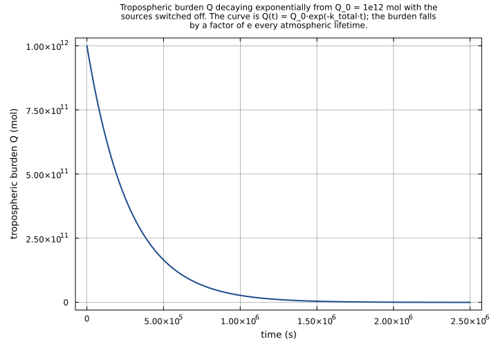
Reproduces the docs figure Exponential Decay from Initial Burden (GasChem.jl docs/src/AtmosphericLifetime.md:450-530). The species starts with a large burden Q_0 = 1.0e12 mol and all source terms are switched off (P_n = P_a = P_c = 0); the burden then decays exponentially under the four default removal pathways. With no production the steady state is an empty troposphere (Q_ss = P_total/k_total = 0), so the burden follows the pure-decay limit Q(t) = Q_0·exp(-k_total·t) of S&P Eq. 2.6, relaxing on the total lifetime tau_total = 1/k_total ≈ 3.2 days. After one lifetime ~37% of the initial burden remains (e^-1); after three lifetimes ~5% (e^-3). The run spans ~9 lifetimes.
Time span: 0.0 → 2500000.0
chemical_loss_sensitivity_sweep
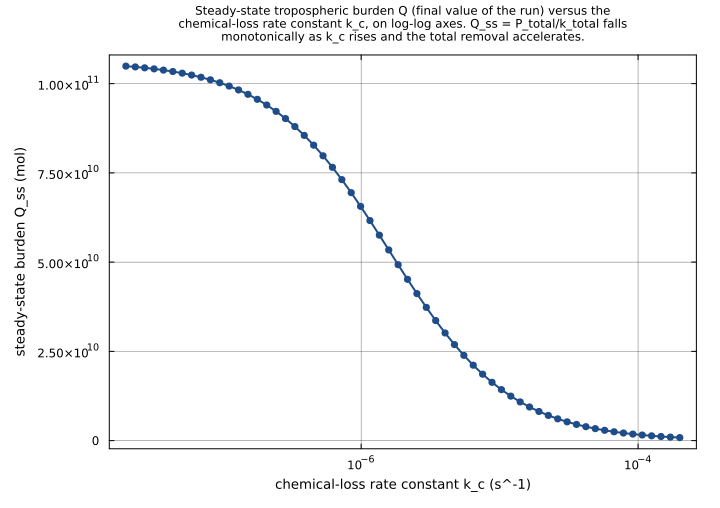
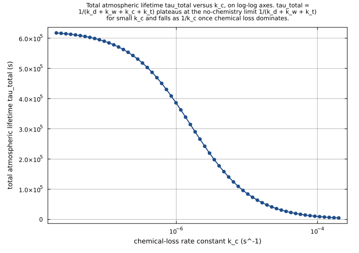
Sweep of the chemical-loss rate constant k_c over four orders of magnitude (2.0e-8 to 2.0e-4 s^-1, logarithmically) with every other parameter at its default and the burden integrated to steady state. As k_c rises, chemical loss goes from a negligible sink (k_c « k_d + k_w + k_t) to the overwhelmingly dominant one (k_c » the rest), so the total lifetime tau_total = 1/(k_d + k_w + k_c + k_t) falls and the steady-state burden Q_ss = P_total/k_total collapses. Illustrates how a single removal pathway controls the budget once its rate constant exceeds the sum of the others — the basis of the S&P observation that the fastest sink sets the atmospheric lifetime.
Time span: 0.0 → 5000000.0
Swept over: k_c
Raw .esm
Raw .esm JSON (this component)
{
"reference": {
"notes": "source_ref: GasChem.jl@280ee50fbc8fb6d8bdf4b12c9ef1c506fe890551:src/AtmosphericLifetime.jl:336\n\nUpstream `TroposphericBudget` is an MTK `@component` declaring four `@parameters` (the first-order removal rate constants k_d, k_w, k_c, k_t, all in s^-1), thirteen time-indexed `@variables` (Q; the three emission/production inputs P_n, P_a, P_c; the diagnostics P_total, R_total, k_total; and the six lifetimes tau_dry, tau_wet, tau_chem, tau_transport, tau_total, tau_production), zero `@constants`, and ten equations (one ODE in Q plus nine algebraic equations). It implements Seinfeld & Pandis (2006) Ch. 2 §2.3 Eqs. 2.13-2.17.\n\nVariable-classification convention: the three emission-input @variables P_n (natural emissions), P_a (anthropogenic emissions), and P_c (in-troposphere chemical production) are encoded here as `type: parameter` because they have no defining equation within the TroposphericBudget component itself — they are externally-supplied source rates. The upstream test suite confirms this directly: both `4.5 TroposphericBudget Compilation` and `5.1 TroposphericBudget ODE Solution` (test/atmospheric_lifetime_test.jl:341-352 and :358-410) compile the component with `mtkcompile(trop; inputs = [trop_nns.P_n, trop_nns.P_a, trop_nns.P_c])` — i.e. P_n/P_a/P_c are passed as `inputs`, which `mtkcompile` resolves into parameters. This mirrors the rig-wide convention applied by sibling oh_production.esm (input @variables O3/H2O/M encoded as `type: parameter`) and ope.esm (input @variables OH/HO2/RO2/NO/NO2 encoded as `type: parameter`). The four declared @parameters k_d/k_w/k_c/k_t carry `type: parameter` directly.\n\nState vs. observed classification: Q is the sole differential state — it is the only variable on the left of a `D(·)` operator (`D(Q) ~ P_total - R_total`, Eq. 2.13), and it is the only entry in the `equations` array. The other nine variables (P_total, R_total, k_total, tau_dry, tau_wet, tau_chem, tau_transport, tau_total, tau_production) are derived quantities: each is defined by exactly one algebraic relation in the inputs, parameters, Q, and (for tau_total, R_total) one another. They are encoded as `type: observed`, each carrying its defining relation in its `expression` field rather than as an `equations` entry. This is the post-`mtkcompile` representation of the upstream system: structural simplification reduces the raw 13-unknown / 10-equation `System(eqs, t)` to a single integrated unknown Q plus nine observed quantities recovered algebraically from Q(t) and the parameters. The 10 upstream relations are preserved exactly as 1 `equations` entry (the Q ODE) + 9 observed `expression` definitions. The encoding matches sibling fastjx.esm (an ODE component with one `state`, one differential `equations` entry, and many `observed` variables) and the observed-only radiation components (stefan_boltzmann.esm, radiation_fundamentals.esm). It is also the robust choice: the per-pathway lifetimes 1/k_X and the production-based lifetime Q/P_total legitimately diverge to +Inf in degenerate regimes (a removal pathway switched off, k_X = 0; or production switched off, P_total = 0 — the configuration of the docs' pure-decay figure). Keeping these nine quantities `observed` keeps the integrator state vector y0 = {Q} finite and the model integrable in every such regime, exactly as the upstream `mtkcompile`d system behaves.\n\nAnalytic solution: with all four removal rate constants and the three source rates held constant, the budget equation dQ/dt = P_total - k_total·Q is a linear first-order ODE with constant coefficients. Its exact solution is Q(t) = Q_ss + (Q_0 - Q_ss)·exp(-k_total·t), where Q_ss = P_total/k_total is the steady-state burden and Q_0 is the initial burden. The e-folding timescale of the relaxation is exactly tau_total = 1/k_total. Every inline-test expected value below is this closed-form analytic solution evaluated at the declared default (or overridden) parameters — the migration is therefore checkable against the textbook formula, not merely against a prior solver run. The diagnostics follow algebraically: R_total = k_total·Q(t), tau_production = Q(t)/P_total, and at t -> infinity R_total -> P_total and tau_production -> tau_total (Eqs. 2.16-2.17: the removal-based and production-based lifetimes coincide at steady state).\n\nNumerical defaults: the upstream @variables and @parameters carry no defaults. The `.esm` defaults are taken from the canonical upstream test/example scenario `5.1 TroposphericBudget ODE Solution` (test/atmospheric_lifetime_test.jl:371-380) and the matching docs figure `Time Evolution of Species Mass` (docs/src/AtmosphericLifetime.md:366-376), a hypothetical reactive species:\n k_d = 1.0e-6 s^-1 (dry deposition, ~11.6 day pathway lifetime)\n k_w = 5.0e-7 s^-1 (wet deposition, ~23.1 day pathway lifetime)\n k_c = 2.0e-6 s^-1 (chemical loss, ~5.8 day pathway lifetime)\n k_t = 1.0e-7 s^-1 (stratospheric transport, ~115.7 day pathway lifetime)\n P_n = 1.0e5 mol/s (natural emissions)\n P_a = 5.0e4 mol/s (anthropogenic emissions)\n P_c = 2.0e4 mol/s (chemical production)\n Q = 0.0 mol (initial burden — the upstream test starts from an empty reservoir)\nAt these defaults P_total = 1.7e5 mol/s, k_total = 3.6e-6 s^-1, tau_total = 1/k_total = 277777.78 s (~3.2 days), and Q_ss = P_total/k_total = 4.7222e10 mol.\n\nUpstream test reproduction:\n- `1.5 TroposphericBudget Structure` (test/atmospheric_lifetime_test.jl:110-140, asserts `length(equations(trop)) == 10`, the four k_d/k_w/k_c/k_t parameters, and the Q/P_n/P_a/P_c/P_total/R_total/tau_* variables) — reproduced by the migrated structural shape: the 10 upstream relations are carried as 1 `equations` entry plus 9 observed `expression` definitions, with 7 parameter + 1 state + 9 observed entries in `variables`. Any structural drift would surface as a load error or an unresolved-variable assertion failure.\n- `2.10 Eq. 2.15: Total Lifetime from Removal` (test/atmospheric_lifetime_test.jl:280-294, k_total = 3.6e-6, tau_total = 277777.78 at the default rate constants) — reproduced and tightened by `initial_conditions_and_lifetime_decomposition`, which pins k_total and tau_total (and every per-pathway lifetime) at rel=1e-10.\n- `4.5 TroposphericBudget Compilation` (test/atmospheric_lifetime_test.jl:341-352, asserts `mtkcompile(trop; inputs=[P_n,P_a,P_c])` returns a `System`) — reproduced implicitly: the migrated `.esm` loads and `mtkcompile`s through the canonical ESS runner before any assertion is evaluated, so every test below presupposes a successful compile.\n- `5.1 TroposphericBudget ODE Solution` (test/atmospheric_lifetime_test.jl:358-410, integrates from Q_0=0 for 10 lifetimes and asserts `Q_final ≈ Q_ss = P_total/k_total` at rtol=0.01) — reproduced and tightened by `upstream_steady_state_approach`, which pins the full Q trajectory at five times spanning the transient plus the steady-state R_total and tau_production at rel=1e-6.\nThe remaining tests extend coverage beyond the upstream suite: the decay branch (Q_0 > Q_ss), equal-pathway lifetime decomposition, emission-source and chemical-sink sensitivities, the minor stratospheric-transport sink, and the production/removal lifetime equivalence at steady state.\n\nTolerance rationale (model-level rel=1.0e-6): the dynamics are a single linear first-order relaxation with one timescale tau_total. The pinned expected values are the exact analytic solution Q(t) = Q_ss + (Q_0 - Q_ss)·exp(-k_total·t); a canonical ESS-runner integration of this linear RHS (Tsit5/Rosenbrock23 at reltol=1e-10, abstol=1e-12 for the Julia walker; LSODA for the Python gate) reproduces it to ~1e-9 relative or better, so rel=1e-6 leaves at least three orders of magnitude of headroom and is far tighter than the upstream test's own rtol=0.01. rel=1e-6 matches the spec §6.6.4 default and the sibling ODE migration nox_cycle.esm. The `initial_conditions_and_lifetime_decomposition` test overrides to rel=1e-10/abs=1e-14 because t=0 carries no integration drift — only the parser->Float64 conversion and the algebraic evaluation of constants. Zero-valued assertions (Q, R_total, tau_production at t=0) carry an abs floor so the degenerate relative comparison against expected=0 is well-posed.\n\nUnit balance (verified): all ten relations balance dimensionally with Q in mol, the source rates P_n/P_a/P_c/P_total/R_total in mol/s, the rate constants k_d/k_w/k_c/k_t/k_total in s^-1, and the lifetimes tau_* in s.\n P_total `P_n + P_a + P_c`: mol/s + mol/s + mol/s = mol/s\n k_total `k_d + k_w + k_c + k_t`: s^-1 + s^-1 + s^-1 + s^-1 = s^-1\n R_total `k_total * Q`: s^-1 · mol = mol/s\n D(Q) `P_total - R_total`: d(mol)/d(s) = mol/s - mol/s = mol/s\n tau_dry/tau_wet/tau_chem/tau_transport `1 / k_X`: 1/(s^-1) = s\n tau_total `1 / k_total`: 1/(s^-1) = s\n tau_production `Q / P_total`: mol/(mol/s) = s\nSI throughout; no unit conversion at parse or runtime."
},
"tolerance": {
"rel": 1e-06
},
"variables": {
"k_d": {
"type": "parameter",
"units": "s^-1",
"default": 1e-06,
"description": "Dry-deposition first-order rate constant (S&P §2.3): removal of the species by uptake at the surface (vegetation, soil, water). The default 1.0e-6 s^-1 corresponds to a dry-deposition pathway lifetime tau_dry = 1/k_d ≈ 11.6 days and is the reactive-species reference value used in the upstream test/example scenario."
},
"k_w": {
"type": "parameter",
"units": "s^-1",
"default": 5e-07,
"description": "Wet-deposition first-order rate constant (S&P §2.3): removal of the species by scavenging into precipitation. The default 5.0e-7 s^-1 corresponds to a wet-deposition pathway lifetime tau_wet = 1/k_w ≈ 23.1 days. Important for soluble species; the smallest-but-one sink in the default scenario."
},
"k_c": {
"type": "parameter",
"units": "s^-1",
"default": 2e-06,
"description": "Chemical-loss first-order rate constant (S&P §2.3): removal of the species by gas-phase reaction (with OH, O3, NO3, photolysis, etc.). The default 2.0e-6 s^-1 corresponds to a chemical-loss pathway lifetime tau_chem = 1/k_c ≈ 5.8 days — the fastest single sink at the default conditions, so it dominates the total removal rate."
},
"k_t": {
"type": "parameter",
"units": "s^-1",
"default": 1e-07,
"description": "Stratospheric-transport first-order rate constant (S&P §2.3): loss of the species from the troposphere by cross-tropopause transport. The default 1.0e-7 s^-1 corresponds to a transport pathway lifetime tau_transport = 1/k_t ≈ 115.7 days — usually the slowest (minor) sink for a tropospheric species."
},
"P_n": {
"type": "parameter",
"units": "mol/s",
"default": 100000.0,
"description": "Natural emission rate [mol/s] (biogenic, volcanic, oceanic, etc.) — an externally-supplied source term. Encoded as `type: parameter` (not `type: observed`) because TroposphericBudget has no governing equation for P_n: the upstream tests compile the component with `mtkcompile(trop; inputs=[P_n, P_a, P_c])`. Contributes to the total production rate P_total = P_n + P_a + P_c."
},
"P_a": {
"type": "parameter",
"units": "mol/s",
"default": 50000.0,
"description": "Anthropogenic emission rate [mol/s] (combustion, industrial, agricultural, etc.) — an externally-supplied source term. Encoded as `type: parameter` for the same reason as P_n. Contributes to the total production rate P_total."
},
"P_c": {
"type": "parameter",
"units": "mol/s",
"default": 20000.0,
"description": "In-troposphere chemical production rate [mol/s] — the rate at which the species is formed by chemistry within the troposphere (e.g. as an oxidation product). An externally-supplied source term, encoded as `type: parameter` for the same reason as P_n. Contributes to the total production rate P_total."
},
"Q": {
"type": "unknown",
"units": "mol",
"default": 0.0,
"description": "Total burden of the species in the troposphere [mol] — the single differential state of the model. Governed by the tropospheric budget equation (S&P Eq. 2.13) D(Q) = P_total - R_total = P_total - k_total·Q. The default initial value 0.0 mol mirrors the upstream test/example scenario, which starts from an empty reservoir and watches the burden grow toward steady state Q_ss = P_total/k_total."
},
"P_total": {
"type": "unknown",
"units": "mol/s",
"description": "Total production rate [mol/s]: the sum of all three source terms, P_total = P_n + P_a + P_c. At the default scenario P_total = 1.7e5 mol/s. Constant in time (the sources are parameters); it sets the numerator of the steady-state burden Q_ss = P_total/k_total and of the production-based lifetime tau_production = Q/P_total."
},
"k_total": {
"type": "unknown",
"units": "s^-1",
"description": "Total first-order removal rate constant [s^-1] (S&P Eq. 2.14): k_total = k_d + k_w + k_c + k_t. The removal rates of independent parallel pathways add. At the default scenario k_total = 3.6e-6 s^-1. Constant in time (the rate constants are parameters); it sets the relaxation timescale of the budget ODE."
},
"R_total": {
"type": "unknown",
"units": "mol/s",
"description": "Total removal rate [mol/s]: R_total = k_total·Q, the first-order loss of the burden across all four removal pathways combined. Grows with the burden as the species accumulates; at steady state R_total -> P_total, so production and removal balance (S&P Eq. 2.2 applied to the troposphere)."
},
"tau_dry": {
"type": "unknown",
"units": "s",
"description": "Dry-deposition pathway lifetime [s] (S&P Eq. 2.6 applied to one pathway): tau_dry = 1/k_d, the lifetime the species would have if dry deposition were its only sink. At the default scenario tau_dry = 1.0e6 s ≈ 11.6 days."
},
"tau_wet": {
"type": "unknown",
"units": "s",
"description": "Wet-deposition pathway lifetime [s]: tau_wet = 1/k_w, the lifetime against wet deposition alone. At the default scenario tau_wet = 2.0e6 s ≈ 23.1 days."
},
"tau_chem": {
"type": "unknown",
"units": "s",
"description": "Chemical-loss pathway lifetime [s]: tau_chem = 1/k_c, the lifetime against chemical loss alone. At the default scenario tau_chem = 5.0e5 s ≈ 5.8 days — the shortest single-pathway lifetime, so chemical loss dominates the total removal."
},
"tau_transport": {
"type": "unknown",
"units": "s",
"description": "Stratospheric-transport pathway lifetime [s]: tau_transport = 1/k_t, the lifetime against cross-tropopause transport alone. At the default scenario tau_transport = 1.0e7 s ≈ 115.7 days — the longest single-pathway lifetime, confirming transport is the minor sink."
},
"tau_total": {
"type": "unknown",
"units": "s",
"description": "Total atmospheric lifetime [s] (S&P Eq. 2.15): tau_total = 1/k_total = 1/(k_d + k_w + k_c + k_t). Because inverse lifetimes add, tau_total is always shorter than the shortest single-pathway lifetime. At the default scenario tau_total ≈ 277777.78 s ≈ 3.2 days. This is the e-folding timescale of the budget ODE's relaxation to steady state."
},
"tau_production": {
"type": "unknown",
"units": "s",
"description": "Production-based lifetime [s] (S&P Eqs. 2.16-2.17): tau_production = Q/P_total, the burden divided by the total production rate. Time-varying because Q evolves; it rises from 0 toward tau_total as the burden relaxes to steady state. At steady state tau_production = Q_ss/P_total = (P_total/k_total)/P_total = 1/k_total = tau_total — the production-based and removal-based lifetimes coincide once production and removal balance."
}
},
"equations": [
{
"lhs": {
"op": "D",
"wrt": "t",
"args": [
"Q"
]
},
"rhs": {
"op": "-",
"args": [
"P_total",
"R_total"
]
}
},
{
"lhs": "P_total",
"rhs": {
"op": "+",
"args": [
"P_n",
"P_a",
"P_c"
]
}
},
{
"lhs": "k_total",
"rhs": {
"op": "+",
"args": [
"k_d",
"k_w",
"k_c",
"k_t"
]
}
},
{
"lhs": "R_total",
"rhs": {
"op": "*",
"args": [
"k_total",
"Q"
]
}
},
{
"lhs": "tau_dry",
"rhs": {
"op": "/",
"args": [
1.0,
"k_d"
]
}
},
{
"lhs": "tau_wet",
"rhs": {
"op": "/",
"args": [
1.0,
"k_w"
]
}
},
{
"lhs": "tau_chem",
"rhs": {
"op": "/",
"args": [
1.0,
"k_c"
]
}
},
{
"lhs": "tau_transport",
"rhs": {
"op": "/",
"args": [
1.0,
"k_t"
]
}
},
{
"lhs": "tau_total",
"rhs": {
"op": "/",
"args": [
1.0,
"k_total"
]
}
},
{
"lhs": "tau_production",
"rhs": {
"op": "/",
"args": [
"Q",
"P_total"
]
}
}
],
"tests": [
{
"id": "initial_conditions_and_lifetime_decomposition",
"description": "At t=0 with every parameter at its declared default the solver must return the empty-reservoir initial state and the exact algebraic diagnostics. Q starts at 0 mol, so the removal rate R_total = k_total·Q and the production-based lifetime tau_production = Q/P_total are both 0. The constant diagnostics are pinned exactly: P_total = 1.7e5 mol/s (= 1e5 + 5e4 + 2e4), k_total = 3.6e-6 s^-1 (= 1e-6 + 5e-7 + 2e-6 + 1e-7), and the per-pathway lifetimes tau_dry = 1e6, tau_wet = 2e6, tau_chem = 5e5, tau_transport = 1e7 s. tau_total = 1/k_total ≈ 277777.78 s reproduces the upstream `2.10 Eq. 2.15: Total Lifetime from Removal` test (atmospheric_lifetime_test.jl:280-294) and confirms the inverse-lifetime sum: 1/tau_total = 1/tau_dry + 1/tau_wet + 1/tau_chem + 1/tau_transport. Tolerance is tightened to rel=1e-10 / abs=1e-14 because t=0 carries no integration drift — only the parser->Float64 conversion and the algebraic constant evaluation. Together with the model loading and compiling successfully, this reproduces the upstream `1.5 TroposphericBudget Structure` test (atmospheric_lifetime_test.jl:110-140).",
"time_span": {
"start": 0.0,
"end": 1.0
},
"tolerance": {
"rel": 1e-10,
"abs": 1e-14
},
"assertions": [
{
"variable": "Q",
"time": 0.0,
"expected": 0.0
},
{
"variable": "P_total",
"time": 0.0,
"expected": 170000.0
},
{
"variable": "k_total",
"time": 0.0,
"expected": 3.6e-06
},
{
"variable": "R_total",
"time": 0.0,
"expected": 0.0
},
{
"variable": "tau_dry",
"time": 0.0,
"expected": 1000000.0
},
{
"variable": "tau_wet",
"time": 0.0,
"expected": 2000000.0
},
{
"variable": "tau_chem",
"time": 0.0,
"expected": 500000.0
},
{
"variable": "tau_transport",
"time": 0.0,
"expected": 10000000.0
},
{
"variable": "tau_total",
"time": 0.0,
"expected": 277777.7777777778
},
{
"variable": "tau_production",
"time": 0.0,
"expected": 0.0
}
]
},
{
"id": "upstream_steady_state_approach",
"description": "Headline behavioral test, the migrated counterpart of the upstream `5.1 TroposphericBudget ODE Solution` test (atmospheric_lifetime_test.jl:358-410) and the docs figure `Time Evolution of Species Mass` (AtmosphericLifetime.md:347-444). Integrate the budget from an empty reservoir (Q_0=0) at the S&P §2.3 default reactive-species parameters for ~9 lifetimes. The burden grows along the exact analytic curve Q(t) = Q_ss·(1 - exp(-k_total·t)) toward the steady state Q_ss = P_total/k_total = 4.7222e10 mol; after one lifetime (t ≈ tau_total ≈ 2.78e5 s) it has reached 1 - 1/e ≈ 63% of Q_ss, and by t = 2.5e6 s (~9 lifetimes) it is within 0.012% of steady state. The upstream test asserts only `Q_final ≈ Q_ss` at rtol=0.01; this test pins the full transient at five times plus the steady-state diagnostics: R_total -> P_total = 1.7e5 mol/s (production balances removal) and tau_production -> tau_total ≈ 277777.78 s (S&P Eqs. 2.16-2.17).",
"time_span": {
"start": 0.0,
"end": 2500000.0
},
"assertions": [
{
"variable": "Q",
"time": 0.0,
"expected": 0.0,
"tolerance": {
"abs": 1e-06
}
},
{
"variable": "Q",
"time": 100000.0,
"expected": 14276395713.312424
},
{
"variable": "Q",
"time": 500000.0,
"expected": 39416441389.53619
},
{
"variable": "Q",
"time": 1000000.0,
"expected": 45931935328.87785
},
{
"variable": "Q",
"time": 2500000.0,
"expected": 47216394537.029236
},
{
"variable": "R_total",
"time": 100000.0,
"expected": 51395.024567924724
},
{
"variable": "R_total",
"time": 2500000.0,
"expected": 169979.02033330523
},
{
"variable": "tau_production",
"time": 2500000.0,
"expected": 277743.4972766426
},
{
"variable": "k_total",
"time": 1000000.0,
"expected": 3.6e-06
},
{
"variable": "tau_total",
"time": 1000000.0,
"expected": 277777.7777777778
}
]
},
{
"id": "decay_from_high_initial_burden",
"description": "Decay branch of the linear relaxation: start from a burden Q_0 = 1.0e12 mol far above the steady state (Q_ss = 4.7222e10 mol) with all parameters at their defaults. The analytic solution Q(t) = Q_ss + (Q_0 - Q_ss)·exp(-k_total·t) now has a positive (Q_0 - Q_ss) coefficient, so the burden decays from 1e12 toward Q_ss as removal outpaces production — the mirror image of `upstream_steady_state_approach`, which approaches the same Q_ss from below. The removal rate R_total = k_total·Q starts high (3.6e6 mol/s, far above the 1.7e5 mol/s production) and falls toward P_total. Exercises the Q_0 > Q_ss sign branch and confirms the steady state is the same attractor regardless of initial burden.",
"time_span": {
"start": 0.0,
"end": 2500000.0
},
"initial_conditions": {
"Q": 1000000000000.0
},
"assertions": [
{
"variable": "Q",
"time": 0.0,
"expected": 1000000000000.0
},
{
"variable": "Q",
"time": 100000.0,
"expected": 711952721784.3434
},
{
"variable": "Q",
"time": 500000.0,
"expected": 204715329611.12277
},
{
"variable": "Q",
"time": 1000000.0,
"expected": 73255657776.17043
},
{
"variable": "Q",
"time": 2500000.0,
"expected": 47339804341.11592
},
{
"variable": "R_total",
"time": 0.0,
"expected": 3600000.0
},
{
"variable": "R_total",
"time": 2500000.0,
"expected": 170423.2956280173
}
]
},
{
"id": "equal_removal_pathways",
"description": "Lifetime-decomposition test with all four removal pathways set to the same rate constant k_d = k_w = k_c = k_t = 1.0e-6 s^-1 (k_w, k_c, k_t overridden up/down to match k_d's default). Each per-pathway lifetime is then identical at tau_X = 1/k_X = 1.0e6 s, while the total lifetime tau_total = 1/k_total = 1/(4·1e-6) = 2.5e5 s is exactly one quarter of each — the N-equal-pathways limit of S&P Eq. 2.15 (the combined lifetime of N identical parallel sinks is the single-pathway lifetime divided by N). Q relaxes from 0 toward Q_ss = P_total/k_total = 1.7e5/4e-6 = 4.25e10 mol. Verifies the inverse-lifetime sum is wired correctly across all four k_X slots.",
"time_span": {
"start": 0.0,
"end": 2500000.0
},
"parameter_overrides": {
"k_w": 1e-06,
"k_c": 1e-06,
"k_t": 1e-06
},
"assertions": [
{
"variable": "k_total",
"time": 0.0,
"expected": 4e-06
},
{
"variable": "tau_total",
"time": 0.0,
"expected": 250000.0
},
{
"variable": "tau_dry",
"time": 0.0,
"expected": 1000000.0
},
{
"variable": "tau_wet",
"time": 0.0,
"expected": 1000000.0
},
{
"variable": "tau_chem",
"time": 0.0,
"expected": 1000000.0
},
{
"variable": "tau_transport",
"time": 0.0,
"expected": 1000000.0
},
{
"variable": "Q",
"time": 250000.0,
"expected": 26865123750.2137
},
{
"variable": "Q",
"time": 1000000.0,
"expected": 41721585347.2288
},
{
"variable": "Q",
"time": 2500000.0,
"expected": 42498070502.98509
}
]
},
{
"id": "emission_source_scaling",
"description": "Source-sensitivity test: raise the anthropogenic emission rate P_a from its default 5.0e4 to 5.0e5 mol/s (10x). The total production rate rises to P_total = P_n + P_a + P_c = 1e5 + 5e5 + 2e4 = 6.2e5 mol/s. Because the removal rate constants are unchanged, the relaxation timescale tau_total ≈ 277777.78 s is identical to the default scenario, but the steady-state burden scales linearly with P_total: Q_ss = P_total/k_total = 6.2e5/3.6e-6 ≈ 1.7222e11 mol, a 3.65x increase tracking the 3.65x rise in P_total. Confirms Q_ss is linear in the emission sources while the lifetime depends only on the sinks.",
"time_span": {
"start": 0.0,
"end": 2500000.0
},
"parameter_overrides": {
"P_a": 500000.0
},
"assertions": [
{
"variable": "P_total",
"time": 0.0,
"expected": 620000.0
},
{
"variable": "tau_total",
"time": 0.0,
"expected": 277777.7777777778
},
{
"variable": "Q",
"time": 500000.0,
"expected": 143754080361.8379
},
{
"variable": "Q",
"time": 2500000.0,
"expected": 172200968311.5184
},
{
"variable": "R_total",
"time": 2500000.0,
"expected": 619923.4859214663
}
]
},
{
"id": "dominant_chemical_sink",
"description": "Sink-sensitivity test: raise the chemical-loss rate constant k_c from its default 2.0e-6 to 2.0e-5 s^-1 (10x). The chemical-loss pathway lifetime shortens to tau_chem = 1/k_c = 5.0e4 s, and chemical loss now overwhelmingly dominates the total removal: k_total = k_d + k_w + k_c + k_t = 1e-6 + 5e-7 + 2e-5 + 1e-7 = 2.16e-5 s^-1, so tau_total = 1/k_total ≈ 46296.3 s — close to tau_chem because the other three pathways are negligible by comparison. The steady-state burden drops to Q_ss = P_total/k_total = 1.7e5/2.16e-5 ≈ 7.870e9 mol (6x below the default Q_ss) and the burden reaches it ~6x faster. Exercises the regime where one sink controls the lifetime.",
"time_span": {
"start": 0.0,
"end": 500000.0
},
"parameter_overrides": {
"k_c": 2e-05
},
"assertions": [
{
"variable": "k_total",
"time": 0.0,
"expected": 2.16e-05
},
{
"variable": "tau_chem",
"time": 0.0,
"expected": 49999.99999999999
},
{
"variable": "tau_total",
"time": 0.0,
"expected": 46296.2962962963
},
{
"variable": "Q",
"time": 100000.0,
"expected": 6962718954.793027
},
{
"variable": "Q",
"time": 500000.0,
"expected": 7870209818.723153
},
{
"variable": "R_total",
"time": 500000.0,
"expected": 169996.53208442012
}
]
},
{
"id": "minor_transport_sink",
"description": "Minor-sink test: drop the stratospheric-transport rate constant k_t from its default 1.0e-7 to 1.0e-8 s^-1 (10x weaker). The transport pathway lifetime lengthens to tau_transport = 1/k_t = 1.0e8 s (~3.2 years), confirming cross-tropopause transport is the slowest sink for a tropospheric species (S&P §2.3). Because k_t was already the smallest of the four rate constants, the total removal barely changes: k_total = 1e-6 + 5e-7 + 2e-6 + 1e-8 = 3.51e-6 s^-1 (only 2.5% below the default 3.6e-6), so tau_total lengthens slightly to ≈ 284900.3 s and Q_ss rises modestly to ≈ 4.843e10 mol. Demonstrates that weakening the minor sink has only a marginal effect on the overall budget.",
"time_span": {
"start": 0.0,
"end": 1000000.0
},
"parameter_overrides": {
"k_t": 1e-08
},
"assertions": [
{
"variable": "k_total",
"time": 0.0,
"expected": 3.51e-06
},
{
"variable": "tau_transport",
"time": 0.0,
"expected": 100000000.0
},
{
"variable": "tau_total",
"time": 0.0,
"expected": 284900.2849002849
},
{
"variable": "Q",
"time": 1000000.0,
"expected": 46985049728.126076
},
{
"variable": "R_total",
"time": 1000000.0,
"expected": 164917.52454572252
}
]
},
{
"id": "production_removal_lifetime_equivalence",
"description": "Steady-state lifetime-equivalence test (S&P Eqs. 2.16-2.17): integrate the default scenario from Q_0=0 for 18 lifetimes (t = 5.0e6 s, k_total·t = 18, exp(-18) ≈ 1.5e-8) so the burden is within ~1.5e-8 of steady state. At this point the burden Q ≈ Q_ss = 4.7222e10 mol, the removal rate R_total ≈ P_total = 1.7e5 mol/s (production and removal balance, S&P Eq. 2.2), and the production-based lifetime tau_production = Q/P_total ≈ tau_total ≈ 277777.78 s — the removal-based lifetime tau_total = 1/k_total and the production-based lifetime tau_production coincide once the system reaches steady state. The pinned expected values are the exact analytic solution at t = 5.0e6 s; each agrees with its steady-state limit to the residual exp(-18) ≈ 1.5e-8, far inside the model rel=1e-6.",
"time_span": {
"start": 0.0,
"end": 5000000.0
},
"assertions": [
{
"variable": "Q",
"time": 5000000.0,
"expected": 47222221503.02873
},
{
"variable": "R_total",
"time": 5000000.0,
"expected": 169999.99741090342
},
{
"variable": "tau_production",
"time": 5000000.0,
"expected": 277777.77354722784
}
]
}
],
"analyses": [
{
"id": "approach_to_steady_state",
"description": "Reproduces the docs figure `Time Evolution of Species Mass` (GasChem.jl docs/src/AtmosphericLifetime.md:347-444). A reactive species is emitted into an initially empty troposphere at the S&P §2.3 default rates and removed by the four parallel sinks. The burden Q grows exponentially at first, then levels off as the removal rate R_total = k_total·Q rises to meet the constant production rate P_total. The characteristic timescale of the approach is the total atmospheric lifetime tau_total = 1/k_total ≈ 3.2 days; after one lifetime the burden has reached 1 - 1/e ≈ 63% of its steady-state value Q_ss = P_total/k_total ≈ 4.72e10 mol. The run spans ~9 lifetimes so the plateau is clearly visible.",
"time_span": {
"start": 0.0,
"end": 2500000.0
},
"plots": [
{
"id": "burden_vs_time",
"type": "line",
"description": "Tropospheric burden Q over time, growing from an empty reservoir toward the steady state Q_ss = P_total/k_total. The curve is the exact relaxation Q(t) = Q_ss·(1 - exp(-k_total·t)); the knee occurs at roughly one atmospheric lifetime.",
"x": {
"variable": "t",
"label": "time (s)"
},
"y": {
"variable": "Q",
"label": "tropospheric burden Q (mol)"
}
},
{
"id": "production_removal_balance_vs_time",
"type": "line",
"description": "Total removal rate R_total over time. It starts at 0 (empty reservoir) and rises toward the constant total production rate P_total = 1.7e5 mol/s; the approach to R_total = P_total is the approach to steady state (S&P Eq. 2.2).",
"x": {
"variable": "t",
"label": "time (s)"
},
"y": {
"variable": "R_total",
"label": "total removal rate R_total (mol/s)"
}
}
]
},
{
"id": "exponential_decay_from_initial_burden",
"description": "Reproduces the docs figure `Exponential Decay from Initial Burden` (GasChem.jl docs/src/AtmosphericLifetime.md:450-530). The species starts with a large burden Q_0 = 1.0e12 mol and all source terms are switched off (P_n = P_a = P_c = 0); the burden then decays exponentially under the four default removal pathways. With no production the steady state is an empty troposphere (Q_ss = P_total/k_total = 0), so the burden follows the pure-decay limit Q(t) = Q_0·exp(-k_total·t) of S&P Eq. 2.6, relaxing on the total lifetime tau_total = 1/k_total ≈ 3.2 days. After one lifetime ~37% of the initial burden remains (e^-1); after three lifetimes ~5% (e^-3). The run spans ~9 lifetimes.",
"time_span": {
"start": 0.0,
"end": 2500000.0
},
"parameters": {
"P_n": 0.0,
"P_a": 0.0,
"P_c": 0.0
},
"initial_state": {
"type": "per_variable",
"values": {
"Q": 1000000000000.0
}
},
"plots": [
{
"id": "decay_vs_time",
"type": "line",
"description": "Tropospheric burden Q decaying exponentially from Q_0 = 1e12 mol with the sources switched off. The curve is Q(t) = Q_0·exp(-k_total·t); the burden falls by a factor of e every atmospheric lifetime.",
"x": {
"variable": "t",
"label": "time (s)"
},
"y": {
"variable": "Q",
"label": "tropospheric burden Q (mol)"
}
}
]
},
{
"id": "chemical_loss_sensitivity_sweep",
"description": "Sweep of the chemical-loss rate constant k_c over four orders of magnitude (2.0e-8 to 2.0e-4 s^-1, logarithmically) with every other parameter at its default and the burden integrated to steady state. As k_c rises, chemical loss goes from a negligible sink (k_c << k_d + k_w + k_t) to the overwhelmingly dominant one (k_c >> the rest), so the total lifetime tau_total = 1/(k_d + k_w + k_c + k_t) falls and the steady-state burden Q_ss = P_total/k_total collapses. Illustrates how a single removal pathway controls the budget once its rate constant exceeds the sum of the others — the basis of the S&P observation that the fastest sink sets the atmospheric lifetime.",
"time_span": {
"start": 0.0,
"end": 5000000.0
},
"parameter_sweep": {
"type": "cartesian",
"dimensions": [
{
"parameter": "k_c",
"range": {
"start": 2e-08,
"stop": 0.0002,
"count": 60,
"scale": "log"
}
}
]
},
"plots": [
{
"id": "steady_state_burden_vs_kc",
"type": "line",
"description": "Steady-state tropospheric burden Q (final value of the run) versus the chemical-loss rate constant k_c, on log-log axes. Q_ss = P_total/k_total falls monotonically as k_c rises and the total removal accelerates.",
"x": {
"variable": "k_c",
"label": "chemical-loss rate constant k_c (s^-1)"
},
"y": {
"variable": "Q",
"label": "steady-state burden Q_ss (mol)"
}
},
{
"id": "total_lifetime_vs_kc",
"type": "line",
"description": "Total atmospheric lifetime tau_total versus k_c, on log-log axes. tau_total = 1/(k_d + k_w + k_c + k_t) plateaus at the no-chemistry limit 1/(k_d + k_w + k_t) for small k_c and falls as 1/k_c once chemical loss dominates.",
"x": {
"variable": "k_c",
"label": "chemical-loss rate constant k_c (s^-1)"
},
"y": {
"variable": "tau_total",
"label": "total atmospheric lifetime tau_total (s)"
}
}
]
}
]
}