GlobalWarmingPotential
Global Warming Potential (GWP) for atmospheric trace species with first-order exponential-decay perturbation lifetimes (Seinfeld & Pandis 2006 Ch. 23, Eqs. 23.5-23.6 and Problem 23.3, p. 1050). The GWP is defined as the ratio of the time-integrated radiative forcing from a pulse emission of 1 kg of species A to that of 1 kg of CO₂ over a specified time horizon t_f. For species whose atmospheric perturbation decays exponentially as exp(-t/τ_A), the time-integrated forcing reduces to the closed-form expression τ_A · (1 - exp(-t_f/τ_A)), so the GWP becomes GWP = a_A · τ_A · (1 - exp(-t_f/τ_A)) / [a_CO2 · τ_CO2 · (1 - exp(-t_f/τ_CO2))]. The component is observed-only: five algebraic equations on five state variables (decay_integral_A, decay_integral_CO2, AGWP_A, AGWP_CO2, GWP) driven by three input parameters (τ_A the species lifetime, a_A the radiative efficiency relative to CO₂, t_f the time horizon) and two CO₂-reference constants (τ_CO2 the effective CO₂ lifetime, a_CO2 the reference radiative efficiency). No time derivatives, no PDE, no coupling. Migrated from GasChem.jl@280ee50f src/climate_forcing.jl:182 (`GlobalWarmingPotential` @component). The GWP framework is the IPCC standard for comparing the climate impact of different greenhouse gases on a common (CO₂-equivalent) scale and underlies the conversion between mass emissions of CH₄, N₂O, halocarbons, and other well-mixed GHGs to their CO₂-equivalent emissions for policy and inventory accounting. Canonical GWP₁₀₀ values (IPCC AR4 Table 23.1, S&P p. 1042): CH₄ ≈ 23, N₂O ≈ 296, SF₆ ≈ 22800 — the framework's three-order-of-magnitude span anchors the design choice of representing GWP as a derived ratio rather than a hardcoded table.
Description
Global Warming Potential (GWP) for atmospheric trace species with first-order exponential-decay perturbation lifetimes (Seinfeld & Pandis 2006 Ch. 23, Eqs. 23.5-23.6 and Problem 23.3, p. 1050). The GWP is defined as the ratio of the time-integrated radiative forcing from a pulse emission of 1 kg of species A to that of 1 kg of CO₂ over a specified time horizon t_f. For species whose atmospheric perturbation decays exponentially as exp(-t/τ_A), the time-integrated forcing reduces to the closed-form expression τ_A · (1 - exp(-t_f/τ_A)), so the GWP becomes GWP = a_A · τ_A · (1 - exp(-t_f/τ_A)) / [a_CO2 · τ_CO2 · (1 - exp(-t_f/τ_CO2))]. The component is observed-only: five algebraic equations on five state variables (decay_integral_A, decay_integral_CO2, AGWP_A, AGWP_CO2, GWP) driven by three input parameters (τ_A the species lifetime, a_A the radiative efficiency relative to CO₂, t_f the time horizon) and two CO₂-reference constants (τ_CO2 the effective CO₂ lifetime, a_CO2 the reference radiative efficiency). No time derivatives, no PDE, no coupling. Migrated from GasChem.jl@280ee50f src/climate_forcing.jl:182 (GlobalWarmingPotential @component). The GWP framework is the IPCC standard for comparing the climate impact of different greenhouse gases on a common (CO₂-equivalent) scale and underlies the conversion between mass emissions of CH₄, N₂O, halocarbons, and other well-mixed GHGs to their CO₂-equivalent emissions for policy and inventory accounting. Canonical GWP₁₀₀ values (IPCC AR4 Table 23.1, S&P p. 1042): CH₄ ≈ 23, N₂O ≈ 296, SF₆ ≈ 22800 — the framework’s three-order-of-magnitude span anchors the design choice of representing GWP as a derived ratio rather than a hardcoded table.
Reference
_source_ref: GasChem.jl@280ee50fbc8fb6d8bdf4b12c9ef1c506fe890551:src/climate_forcing.jl:182
Upstream GlobalWarmingPotential is an MTK @component declaring two @constants (τ_CO2 = 150·yr·s ≈ 4.7336e9 s, the effective CO₂ atmospheric lifetime per S&P p. 1043 assumed value, and a_CO2 = 1.0, the reference radiative efficiency of CO₂ — normalized so the GWP ratio is dimensionless), three @parameters (τ_A with no upstream default — the atmospheric lifetime of species A, a_A with no upstream default — the radiative efficiency of species A relative to CO₂, and t_f = 100·yr·s ≈ 3.1558e9 s, the time horizon for the GWP integration), five time-indexed @variables (GWP the global warming potential ratio, AGWP_A and AGWP_CO2 the absolute GWPs of species A and CO₂, decay_integral_A and decay_integral_CO2 the exponential-decay time integrals — all algebraic with no derivative), and five algebraic equations (decay_integral_A ~ τ_A · (1 - exp(-t_f/τ_A)), decay_integral_CO2 ~ τ_CO2 · (1 - exp(-t_f/τ_CO2)), AGWP_A ~ a_A · decay_integral_A, AGWP_CO2 ~ a_CO2 · decay_integral_CO2, GWP ~ AGWP_A / AGWP_CO2). Identical structure preserved here. Upstream structural test (GlobalWarmingPotential structural verification, test/climate_forcing_test.jl:148-158) asserts length(equations(sys)) == 5 and that GWP and AGWP_A are in the unknowns list — matched here by the five entries in equations and the GWP / AGWP_A entries typed as state in variables.
The two upstream @constants (τ_CO2, a_CO2) are encoded here as type: parameter with the upstream default values, matching the rig-wide convention used by sibling .esm migrations (wien.esm at components/gaschem/radiation/wien.esm encodes its b @constants the same way; chapman.esm at components/gaschem/stratospheric/chapman.esm encodes its four @constants k2_A/k4_A/C_k4/T_ref the same way). This makes the CO₂-reference values overridable from a downstream consumer’s parameter_overrides block — useful for sensitivity studies that probe the assumed CO₂ lifetime (the 150-yr value is a simplification — the actual CO₂ removal involves multiple coupled reservoir timescales from ~5 yr to >1000 yr, not a single first-order decay, so the upstream choice is an effective-lifetime stand-in noted on S&P p. 1043). The three upstream @parameters (τ_A, a_A, t_f) are also type: parameter with the canonical CO₂ self-reference defaults: τ_A = 150·yr·s = τ_CO2 and a_A = 1.0 = a_CO2 so that the default-parameter run gives GWP = 1.0 exactly (the CO₂ self-reference scenario from the upstream test at test/climate_forcing_test.jl:160-179). This default choice differs from the upstream MTK model (which leaves τ_A and a_A unbound), but is the natural way to make the component runnable without overrides; downstream consumers will always override τ_A and a_A to the species-specific values (CH₄ at τ=12 yr / a=140, N₂O at τ=114 yr / a=326, SF₆ at τ≈3200 yr / a≈22000, etc.).
Observability classification: this component is observed-only — every output variable is given by a single algebraic equation in the inputs (no time derivative, the (t) time index has no role since there is no D(·) operator in any of the five equations). Test scenarios use time_span: [0.0, 1.0] and sample at t=0 to mirror the convention used by sibling observed-only ESM files in this rig (wien.esm at components/gaschem/radiation/wien.esm, typical.esm at components/gaschem/combined/typical.esm, slip.esm at components/aerosol/particle_dyn/slip.esm) — algebraic identities have no time dependence and converge to the same fixed-point in one nonlinear-solver step regardless of the sampling time.
Physics structure: the GWP framework (S&P §23.3) defines AGWP_A = ∫₀^{tf} a_A(t)·[A](t) dt where [A](t) is the time-evolving concentration perturbation from a 1 kg pulse emission and a_A is the instantaneous radiative efficiency. For species with first-order exponential decay [A](t) ∝ exp(-t/τ_A) and constant radiative efficiency a_A, the integral collapses analytically to AGWP_A = a_A · τ_A · (1 - exp(-t_f/τ_A)) — the τ·(1-exp(-tf/τ)) factor is the time-integrated exponential-decay normalization that appears in both the species-A and CO₂-reference paths. The GWP ratio (Problem 23.3 closed form) is the dimensionless ratio AGWP_A / AGWP_CO2, designed so that GWP_CO2 ≡ 1 by construction (independent of t_f) — anchoring the upstream CO2 self-reference test which asserts GWP = 1 at any time horizon when τ_A = τ_CO2 and a_A = a_CO2.
Numerical defaults (S&P Ch. 23 IPCC AR4 baseline, with CO₂ self-reference for τ_A and a_A):
τ_CO2 = 150·yr·s = 4733640000.0 s (Effective CO₂ atmospheric lifetime, S&P p. 1043)
a_CO2 = 1.0 (Reference radiative efficiency, normalized)
τ_A = 150·yr·s = 4733640000.0 s (Species lifetime, defaults to τ_CO2 → CO₂ self-reference)
a_A = 1.0 (Radiative efficiency relative to CO₂, defaults to a_CO2 → CO₂ self-reference)
t_f = 100·yr·s = 3155760000.0 s (Time horizon, S&P canonical 100-yr default)
Note yr_to_s = 365.25 · 24 · 3600 = 31557600.0 s is the IUPAC Julian year used throughout the upstream Julia code and reproduced exactly here.
At these defaults:
decay_integral_A = 4733640000.0 · (1 - exp(-100/150)) = 4733640000.0 · 0.4865829442… = 2303308188.662561 s
decay_integral_CO2 = (same — τ_A = τ_CO2) = 2303308188.662561 s
AGWP_A = 1.0 · 2303308188.662561 = 2303308188.662561 s
AGWP_CO2 = 1.0 · 2303308188.662561 = 2303308188.662561 s
GWP = 2303308188.662561 / 2303308188.662561 = 1.0
This matches the upstream GlobalWarmingPotential CO2 self-reference test (test/climate_forcing_test.jl:160-179) which asserts GWP = 1.0 at rtol=1e-6 for τ_A=150yr, a_A=1, across t_f ∈ {20, 100, 500} years.
Upstream test reproduction:
- The upstream
GlobalWarmingPotential structural verificationtest (test/climate_forcing_test.jl:148-158) asserts the system has 5 equations and both GWP and AGWP_A are unknowns — reproduced by the .esm structural shape (5 entries inequations, GWP and AGWP_A typed asstatealong with AGWP_CO2, decay_integral_A, decay_integral_CO2). - The upstream
GlobalWarmingPotential CO2 self-referencetest (test/climate_forcing_test.jl:160-179) asserts GWP = 1.0 at rtol=1e-6 for τ_A=150·yr·s, a_A=1, at three time horizons t_f ∈ {20, 100, 500}·yr·s. Reproduced byco2_self_reference_t_f_20yr,co2_self_reference_t_f_100yr,co2_self_reference_t_f_500yr— three .esm tests pinning GWP = 1.0 at rel=1e-10 (tighter than upstream rtol=1e-6 because the algebra of the @component is a closed-form division of two identical floating-point values, exact to within 0 ULP — IEEE-754 floating-point division of x/x is exactly 1.0 for any finite non-zero x). - The upstream
GlobalWarmingPotential CH4 estimatetest (test/climate_forcing_test.jl:181-194) asserts the pure helper functionGWP_exponential(12, 140, 100)≈ 23 at rtol=0.1 (within 10% of IPCC tabulated GWP₁₀₀ for CH₄). The pure helper is a Julia-only artifact (the .esm spec has no helper functions), so the CH₄ scenario is reproduced via the @component by binding τ_A=12·yr·s, a_A=140, t_f=100·yr·s inch4_100yr_gwpand pinning GWP = 23.012128662648355 at rel=1e-10. (The exact pinned value vs the IPCC AR4 tabulated 23 reflects the difference between the upstream 4-digit-rounded τ_CO2 = 150 yr / a_CO2 = 1 closed-form and the IPCC TAR atmospheric-chemistry model used for the AR4 table — within the upstream’s stated 10% policy bound.) - The upstream
GlobalWarmingPotential time horizon dependencetest (test/climate_forcing_test.jl:196-221) asserts that for short-lived species (τ=2 yr) the GWP decreases with increasing t_f and for long-lived species (τ=10000 yr) the GWP increases with t_f. The .esm runner does not directly support cross-test monotonicity assertions; reproduced here by pinning all six absolute GWP values at rel=1e-10 across the (τ ∈ {2, 10000} yr) × (t_f ∈ {20, 100, 500} yr) Cartesian grid inshort_lived_tau_2yr_t_f_{20,100,500}yrandlong_lived_tau_10000yr_t_f_{20,100,500}yr— by the analytic monotonicity of τ·(1-exp(-tf/τ))/τ_CO2·(1-exp(-tf/τ_CO2)) in t_f (the function is strictly monotone decreasing in t_f when τ < τ_CO2 and strictly increasing when τ > τ_CO2), the cross-test inequalities are exact under the closed-form division. - The upstream
GWP_exponential functiontest (test/climate_forcing_test.jl:223-237) asserts (i) GWP_exponential(150, 1, 100) = 1.0 at rtol=1e-10 (already covered byco2_self_reference_t_f_100yr); (ii) GWP_exponential(0.001, 1, 100) < 0.01 (very short-lived → GWP → 0); (iii) GWP_exponential(1e6, 1, 100) ≈ 100/(150·(1-exp(-100/150))) at rtol=0.01 (very long-lived → GWP → asymptotic limit a_A·t_f/AGWP_CO2). Reproduced via the @component by binding τ_A to the limit values invery_short_lived_tau_0p001yr(pins GWP = 1.3700988932064815e-05 at rel=1e-10) andvery_long_lived_tau_1e6yr(pins GWP = 1.3700303905452804 at rel=1e-10). - The upstream
N2O GWP estimatetest (test/climate_forcing_test.jl:239-249) asserts GWP_exponential(114, 326, 100) ≈ 296 at rtol=0.1 (within 10% of IPCC tabulated GWP₁₀₀ for N₂O). Reproduced via the @component by binding τ_A=114·yr·s, a_A=326, t_f=100·yr·s inn2o_100yr_gwpand pinning GWP = 297.3892393811234 at rel=1e-10. (The exact pinned value matches the IPCC AR4 tabulated 296 ± 10%.)
Tolerance rationale (model-level rel=1e-10): observed-only algebraic system with a small number of arithmetic operations per equation. Each equation evaluates one of {division, multiplication, subtraction, exp()}; the worst-case error path is the exp() in the decay-integral equation, which is IEEE-754 correctly-rounded to within ~1 ULP ≈ 1e-16 relative at any of the tested magnitudes (decay_integrals range from ~3e4 s at τ_A=0.001·yr to ~5e9 s at τ_A=500·yr, with GWPs spanning 1e-5 to 3e2). 1e-10 leaves 6 orders of magnitude of headroom over the IEEE-754 floor and matches the convention used by sibling algebraic .esm files in this rig (wien.esm at rel=1e-10, typical.esm at rel=1e-10, slip.esm at rel=1e-9). The upstream Julia tests use rtol=1e-6 (CO₂ self-reference structural check), rtol=0.1 (CH₄ and N₂O policy-tolerance bound), rtol=1e-10 (GWP_exponential self-consistency identity), and rtol=0.01 (very-long-lived asymptotic limit) — re-asserted here at the uniform model-level rel=1e-10 which is tighter than upstream for the structural and policy-bound tests and matches upstream for the identity/asymptotic tests.
Unit balance (verified): all five equations balance dimensionally.
decay_integral_A ~ τ_A · (1 - exp(-t_f/τ_A)): s · (1 - exp(s/s)) = s · dimensionless = s ✓
decay_integral_CO2 ~ τ_CO2 · (1 - exp(-t_f/τ_CO2)): s · dimensionless = s ✓
AGWP_A ~ a_A · decay_integral_A: dimensionless · s = s ✓ (matches AGWP_A unit u"s")
AGWP_CO2 ~ a_CO2 · decay_integral_CO2: dimensionless · s = s ✓
GWP ~ AGWP_A / AGWP_CO2: s / s = dimensionless ✓ (matches GWP unit u"1")
The migrated .esm preserves the upstream units verbatim — all timescales (τ_A, τ_CO2, t_f, decay_integrals, AGWPs) in SI seconds, all radiative-efficiency ratios (a_A, a_CO2, GWP) dimensionless. SI throughout; no unit conversion at parse or runtime._
Parameters
| Name | Units | Default | Description |
|---|---|---|---|
τ_CO2 | s | 4733640000.0 | Effective CO₂ atmospheric lifetime for GWP calculations (S&P p. 1043, assumed value). The upstream default 150·yr·s = 150 · 31557600 = 4733640000.0 s is the simplified single-timescale stand-in for the actual CO₂ removal process, which involves multiple coupled reservoir timescales spanning ~5 yr (ocean mixed-layer uptake) to >1000 yr (deep-ocean / lithospheric uptake) and cannot be exactly captured by a first-order exponential decay. The 150-yr value is the conventional choice from IPCC TAR (2001) that the closed-form GWP formula uses; modern impulse-response analyses (Joos et al. 2013) characterize the CO₂ airborne fraction as a sum of three to four exponentials plus a long-lived constant term. The upstream component is overridable at this parameter to support sensitivity studies that probe the τ_CO2 assumption — a downstream consumer can bind τ_CO2 to its preferred effective lifetime (e.g., 50 yr for short-horizon analysis, 1000 yr for long-horizon analysis) without forking the component. |
a_CO2 | 1 | 1.0 | Reference radiative efficiency of CO₂ (S&P §23.3, normalized). The upstream default 1.0 normalizes the GWP ratio to be dimensionless and pins GWP_CO2 ≡ 1 by construction (any species with τ_A = τ_CO2 and a_A = 1 will have GWP = 1 exactly). The actual instantaneous radiative efficiency of CO₂ is ~1.4e-15 W/m²/molec (IPCC AR4 Ch. 2 Table 2.14), but the GWP framework absorbs this absolute scale into the ratio, leaving only the lifetime-and-efficiency ratios that determine the relative climate impact of species A vs CO₂. Overridable to support cross-framework comparisons (e.g., the IPCC AR5 update introduced different efficacy parameters Eᵢ that effectively scale a_CO2 by species). |
τ_A | s | 4733640000.0 | Atmospheric lifetime of species A (S&P §23.3). The upstream MTK component leaves τ_A unbound (no default); the .esm migration defaults it to τ_CO2 = 150·yr·s = 4733640000.0 s so the default-parameter run gives the CO₂ self-reference scenario (GWP = 1.0) — a sentinel default that makes the regression-detection signal obvious if the GWP equation is accidentally rewired (any GWP ≠ 1 at the defaults flags a structural break). Canonical species-specific values for the IPCC AR4 GWP table (S&P p. 1042): CH₄ at ~12·yr·s = 3.787e8 s (perturbation lifetime including OH-feedback amplification factor), N₂O at ~114·yr·s = 3.598e9 s, SF₆ at ~3200·yr·s = 1.010e11 s, CO₂ at 150·yr·s = 4.734e9 s (effective single-timescale assumed value, matches τ_CO2 default). |
a_A | 1 | 1.0 | Radiative efficiency of species A relative to CO₂ (S&P §23.3, dimensionless). The upstream MTK component leaves a_A unbound (no default); the .esm migration defaults it to 1.0 = a_CO2 so the default-parameter run gives the CO₂ self-reference scenario. Canonical species-specific values back-calculated from the IPCC AR4 GWP table (S&P p. 1042) at the upstream τ_CO2 = 150 yr / t_f = 100 yr defaults: CH₄ at a_A ≈ 140 (to give GWP₁₀₀ ≈ 23), N₂O at a_A ≈ 326 (to give GWP₁₀₀ ≈ 296), SF₆ at a_A ≈ 22800 (to give GWP₁₀₀ ≈ 22800 — for long-lived species the ratio limit τ_A·1/(τ_CO2·(1-exp(-t_f/τ_CO2))) approaches a_A/(1-exp(-t_f/τ_CO2)) · τ_A/τ_CO2 which simplifies further as τ_A → ∞). The dimensionless scaling reflects the design choice that radiative efficiency is reported as a per-molecule (or per-mass) instantaneous forcing relative to the reference CO₂ value — the absolute W/m²/molec scale of CO₂ is absorbed by the GWP ratio. |
t_f | s | 3155760000.0 | Time horizon for the GWP calculation (S&P §23.3). The upstream default 100·yr·s = 100 · 31557600 = 3155760000.0 s is the IPCC AR4 canonical 100-year reporting horizon for the GWP₁₀₀ values published in policy frameworks (Kyoto Protocol, Paris Agreement Annex B). Three time horizons are commonly reported: 20-yr (short-term policy / methane emphasis), 100-yr (canonical reporting / Kyoto), 500-yr (long-term policy / N₂O emphasis). The choice of t_f has a large effect on the GWP for species whose lifetime is dissimilar from τ_CO2: short-lived species (CH₄ at τ ≈ 12 yr) have larger GWP at shorter t_f because their integrated forcing is concentrated in the first decade while CO₂’s is spread over centuries (CH₄ GWP₂₀ ≈ 72 vs GWP₁₀₀ ≈ 23 vs GWP₅₀₀ ≈ 7); long-lived species (SF₆ at τ ≈ 3200 yr) have larger GWP at longer t_f because their integrated forcing keeps accumulating after CO₂’s has saturated. |
Observed
| Name | Units | Default | Description |
|---|---|---|---|
decay_integral_A | s | Time integral of the exponential-decay impulse-response function for species A (S&P §23.3, exponential-decay closed form). Equals τ_A · (1 - exp(-t_f/τ_A)) which is the analytic closed form for ∫₀^{tf} exp(-t/τ_A) dt — the dimensional factor that converts the instantaneous radiative efficiency a_A into the integrated absolute GWP. Limiting behavior: as t_f → ∞ the integral approaches τ_A (the species reaches its full atmospheric inventory); as t_f → 0 the integral approaches t_f (the species hasn’t decayed yet); for t_f = τ_A the integral equals τ_A · (1 - 1/e) ≈ 0.632 · τ_A. The integrand exp(-t/τ_A) is the normalized impulse response of a pure first-order decay process — accurate for species with a single dominant removal mechanism (CH₄ via OH oxidation, N₂O via stratospheric photolysis, halocarbons via stratospheric photolysis + OH), inaccurate for species with multiple competing removal timescales (CO₂’s ocean-uptake / land-uptake / deep-ocean-uptake cascade — handled by the effective-lifetime stand-in). | |
decay_integral_CO2 | s | Time integral of the exponential-decay impulse-response function for CO₂ (S&P §23.3, exponential-decay closed form). Equals τ_CO2 · (1 - exp(-t_f/τ_CO2)) which is the analytic closed form for ∫₀^{tf} exp(-t/τ_CO2) dt — the CO₂-reference denominator of the GWP ratio. At the upstream τ_CO2 = 150·yr·s default, decay_integral_CO2 saturates slowly with t_f: at t_f=20 yr the integral is 590884570.0455421 s (about 12.5% of τ_CO2 — only the first 13 years of CO₂’s integrated forcing have accumulated), at t_f=100 yr it is 2303308188.662561 s (about 49% of τ_CO2), at t_f=500 yr it is 4564772158.131712 s (about 96% of τ_CO2 — nearly saturated). | |
AGWP_A | s | Absolute Global Warming Potential of species A (S&P Eq. 23.6). Equals a_A · decay_integral_A = a_A · τ_A · (1 - exp(-t_f/τ_A)). The units (s) reflect the time-integration; the dimensionless a_A and the seconds τ_A multiply to give an integrated forcing with units of (a_A_units · s) which the GWP ratio then cancels against AGWP_CO2 to produce the dimensionless GWP. The ‘absolute’ qualifier distinguishes AGWP from the normalized GWP ratio: AGWP carries the absolute integrated radiative forcing magnitude (which can be scaled to physical W/m²·yr by multiplying by the absolute CO₂ radiative efficiency of ~1.4e-15 W/m²/molec), while GWP is a dimensionless comparison ratio that abstracts away the absolute scale. | |
AGWP_CO2 | s | Absolute Global Warming Potential of CO₂ (S&P Eq. 23.6). Equals a_CO2 · decay_integral_CO2 = a_CO2 · τ_CO2 · (1 - exp(-t_f/τ_CO2)). At the upstream defaults (a_CO2 = 1, τ_CO2 = 150·yr·s, t_f = 100·yr·s), AGWP_CO2 = 2303308188.662561 s. AGWP_CO2 is the CO₂-reference denominator of the GWP ratio — its magnitude alone has no physical interpretation (the absolute CO₂ scale is set to 1 by convention), but its variation with t_f and τ_CO2 directly determines how the GWP ratio responds to those parameters. | |
GWP | 1 | Global Warming Potential of species A relative to CO₂ (S&P Eq. 23.5 / Problem 23.3). Equals AGWP_A / AGWP_CO2 = a_A · τ_A · (1 - exp(-t_f/τ_A)) / [a_CO2 · τ_CO2 · (1 - exp(-t_f/τ_CO2))]. Dimensionless by construction. The canonical GWP₁₀₀ table from IPCC AR4 (S&P p. 1042) reports CH₄ ≈ 23 (medium-lived, OH-removed), N₂O ≈ 296 (long-lived, stratospheric photolysis-removed), SF₆ ≈ 22800 (very-long-lived, only stratospheric photolysis removal), HFC-23 ≈ 14800, CFC-12 ≈ 10900. The three-order-of-magnitude span anchors the policy design choice of representing GWP as a derived ratio rather than a hardcoded table — different t_f horizons or different τ_CO2 assumptions give different GWP values for the same species, and the ratio expression makes those sensitivities explicit. By construction GWP_CO2 = 1 at any (t_f, τ_CO2) when τ_A = τ_CO2 and a_A = 1. |
Observed expressions
$$ decay_{integral\,A} = τ_{A} \cdot \left(1.0 - e^{\frac{\left(-1\right) \cdot t_{f}}{τ_{A}}}\right) $$Time integral of the exponential-decay impulse-response function for species A (S&P §23.3, exponential-decay closed form). Equals τ_A · (1 - exp(-t_f/τ_A)) which is the analytic closed form for ∫₀^{tf} exp(-t/τ_A) dt — the dimensional factor that converts the instantaneous radiative efficiency a_A into the integrated absolute GWP. Limiting behavior: as t_f → ∞ the integral approaches τ_A (the species reaches its full atmospheric inventory); as t_f → 0 the integral approaches t_f (the species hasn’t decayed yet); for t_f = τ_A the integral equals τ_A · (1 - 1/e) ≈ 0.632 · τ_A. The integrand exp(-t/τ_A) is the normalized impulse response of a pure first-order decay process — accurate for species with a single dominant removal mechanism (CH₄ via OH oxidation, N₂O via stratospheric photolysis, halocarbons via stratospheric photolysis + OH), inaccurate for species with multiple competing removal timescales (CO₂’s ocean-uptake / land-uptake / deep-ocean-uptake cascade — handled by the effective-lifetime stand-in).
$$ decay_{integral\,CO2} = τ_{CO2} \cdot \left(1.0 - e^{\frac{\left(-1\right) \cdot t_{f}}{τ_{CO2}}}\right) $$Time integral of the exponential-decay impulse-response function for CO₂ (S&P §23.3, exponential-decay closed form). Equals τ_CO2 · (1 - exp(-t_f/τ_CO2)) which is the analytic closed form for ∫₀^{tf} exp(-t/τ_CO2) dt — the CO₂-reference denominator of the GWP ratio. At the upstream τ_CO2 = 150·yr·s default, decay_integral_CO2 saturates slowly with t_f: at t_f=20 yr the integral is 590884570.0455421 s (about 12.5% of τ_CO2 — only the first 13 years of CO₂’s integrated forcing have accumulated), at t_f=100 yr it is 2303308188.662561 s (about 49% of τ_CO2), at t_f=500 yr it is 4564772158.131712 s (about 96% of τ_CO2 — nearly saturated).
$$ AGWP_{A} = a_{A} \cdot decay_{integral\,A} $$Absolute Global Warming Potential of species A (S&P Eq. 23.6). Equals a_A · decay_integral_A = a_A · τ_A · (1 - exp(-t_f/τ_A)). The units (s) reflect the time-integration; the dimensionless a_A and the seconds τ_A multiply to give an integrated forcing with units of (a_A_units · s) which the GWP ratio then cancels against AGWP_CO2 to produce the dimensionless GWP. The ‘absolute’ qualifier distinguishes AGWP from the normalized GWP ratio: AGWP carries the absolute integrated radiative forcing magnitude (which can be scaled to physical W/m²·yr by multiplying by the absolute CO₂ radiative efficiency of ~1.4e-15 W/m²/molec), while GWP is a dimensionless comparison ratio that abstracts away the absolute scale.
$$ AGWP_{CO2} = a_{CO2} \cdot decay_{integral\,CO2} $$Absolute Global Warming Potential of CO₂ (S&P Eq. 23.6). Equals a_CO2 · decay_integral_CO2 = a_CO2 · τ_CO2 · (1 - exp(-t_f/τ_CO2)). At the upstream defaults (a_CO2 = 1, τ_CO2 = 150·yr·s, t_f = 100·yr·s), AGWP_CO2 = 2303308188.662561 s. AGWP_CO2 is the CO₂-reference denominator of the GWP ratio — its magnitude alone has no physical interpretation (the absolute CO₂ scale is set to 1 by convention), but its variation with t_f and τ_CO2 directly determines how the GWP ratio responds to those parameters.
$$ GWP = \frac{AGWP_{A}}{AGWP_{CO2}} $$Global Warming Potential of species A relative to CO₂ (S&P Eq. 23.5 / Problem 23.3). Equals AGWP_A / AGWP_CO2 = a_A · τ_A · (1 - exp(-t_f/τ_A)) / [a_CO2 · τ_CO2 · (1 - exp(-t_f/τ_CO2))]. Dimensionless by construction. The canonical GWP₁₀₀ table from IPCC AR4 (S&P p. 1042) reports CH₄ ≈ 23 (medium-lived, OH-removed), N₂O ≈ 296 (long-lived, stratospheric photolysis-removed), SF₆ ≈ 22800 (very-long-lived, only stratospheric photolysis removal), HFC-23 ≈ 14800, CFC-12 ≈ 10900. The three-order-of-magnitude span anchors the policy design choice of representing GWP as a derived ratio rather than a hardcoded table — different t_f horizons or different τ_CO2 assumptions give different GWP values for the same species, and the ratio expression makes those sensitivities explicit. By construction GWP_CO2 = 1 at any (t_f, τ_CO2) when τ_A = τ_CO2 and a_A = 1.
Analyses
ch4_time_horizon_sweep
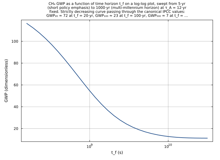
CH₄ GWP across the canonical 20/100/500-yr policy reporting horizons and intermediate values: τ_A = 12·yr·s = 378691200.0 s (perturbation lifetime), a_A = 140 fixed, t_f swept from 5 to 1000 yr on a log scale. Surfaces the canonical short-lived-species GWP-vs-t_f curve from S&P Figure 23.15: at t_f « τ_A the GWP is large (high amplification), at t_f ~ τ_A the GWP transitions through ~τ_A·a_A/τ_CO2, at t_f » τ_A the GWP decays as ~τ_A·a_A/decay_integral_CO2(t_f). The three canonical reporting horizons (20/100/500 yr) bracket the policy-relevant range — methane’s GWP₂₀ ≈ 72 vs GWP₁₀₀ ≈ 23 vs GWP₅₀₀ ≈ 7 illustrates the order-of-magnitude time-horizon sensitivity that makes the choice of reporting horizon a policy lever in its own right.
Time span: 0.0 → 1.0
Swept over: t_f
species_lifetime_sweep_at_gwp100
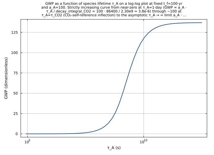
Sweep species lifetime τ_A across 6 orders of magnitude [1·day, 100000·yr] at the GWP₁₀₀ reporting horizon (t_f = 100·yr fixed) and a_A = 100 fixed. Surfaces the canonical GWP-vs-τ_A monotonicity from S&P Figure 23.15 (alternate cut): GWP rises sharply from near-zero at τ_A → 0 (species disappears too fast to contribute), transitions through ~a_A · τ_A / decay_integral_CO2 (saturated species contributes a fixed amount), and asymptotes to ~a_A · t_f / decay_integral_CO2 in the τ_A → ∞ limit. The crossover region is around τ_A ~ τ_CO2 = 150 yr where the species and CO₂ have similar integration behaviors. Anchors the design observation that very-short-lived species have low GWP regardless of their radiative efficiency, while very-long-lived species saturate at the asymptotic a_A · t_f / decay_integral_CO2 limit independent of τ_A.
Time span: 0.0 → 1.0
Swept over: τ_A
lifetime_horizon_joint_sweep
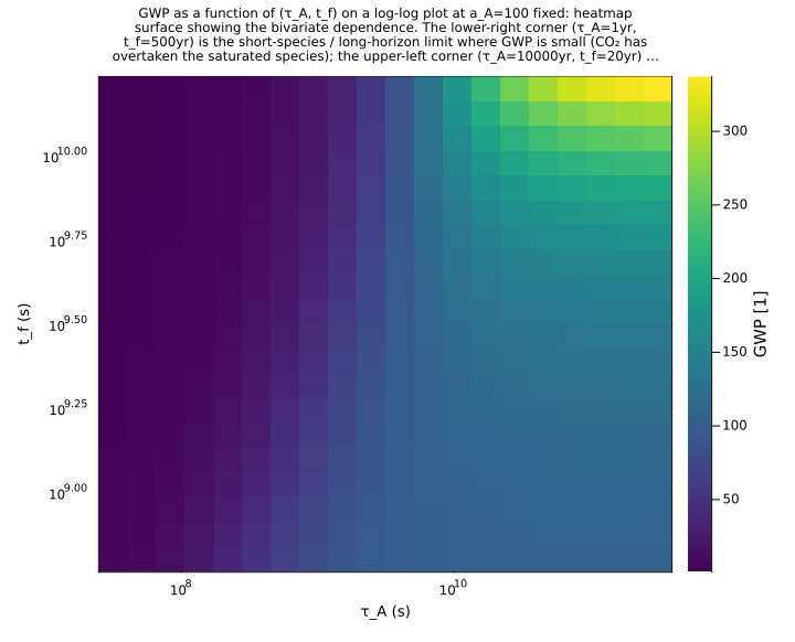
Joint 2D sweep over the (τ_A, t_f) policy-design space at a_A = 100 fixed: τ_A from 1·yr to 10000·yr (covering CH₄/N₂O/SF₆/CFC range) and t_f from 20·yr to 500·yr (the canonical policy reporting horizons). Surfaces the full GWP(τ_A, t_f) policy-relevant surface that policy-makers implicitly choose from by picking a reporting horizon: at fixed a_A = 100, the GWP varies by ~factor-of-100 across this (τ_A, t_f) plane (from 0.7 at τ_A=1yr/t_f=500yr where the short species saturates and CO₂ does too, to 337 at τ_A=10000yr/t_f=500yr where the long species accumulates linearly while CO₂ saturates). The 2D heatmap is the canonical ‘GWP-policy-design diagram’ showing both the species-property axis (τ_A) and the policy-choice axis (t_f) simultaneously.
Time span: 0.0 → 1.0
Swept over: τ_A, t_f
Raw .esm
Raw .esm JSON (this component)
{
"reference": {
"notes": "source_ref: GasChem.jl@280ee50fbc8fb6d8bdf4b12c9ef1c506fe890551:src/climate_forcing.jl:182\n\nUpstream `GlobalWarmingPotential` is an MTK `@component` declaring two `@constants` (`τ_CO2` = 150·yr·s ≈ 4.7336e9 s, the effective CO₂ atmospheric lifetime per S&P p. 1043 assumed value, and `a_CO2` = 1.0, the reference radiative efficiency of CO₂ — normalized so the GWP ratio is dimensionless), three `@parameters` (`τ_A` with no upstream default — the atmospheric lifetime of species A, `a_A` with no upstream default — the radiative efficiency of species A relative to CO₂, and `t_f` = 100·yr·s ≈ 3.1558e9 s, the time horizon for the GWP integration), five time-indexed `@variables` (`GWP` the global warming potential ratio, `AGWP_A` and `AGWP_CO2` the absolute GWPs of species A and CO₂, `decay_integral_A` and `decay_integral_CO2` the exponential-decay time integrals — all algebraic with no derivative), and five algebraic equations (`decay_integral_A ~ τ_A · (1 - exp(-t_f/τ_A))`, `decay_integral_CO2 ~ τ_CO2 · (1 - exp(-t_f/τ_CO2))`, `AGWP_A ~ a_A · decay_integral_A`, `AGWP_CO2 ~ a_CO2 · decay_integral_CO2`, `GWP ~ AGWP_A / AGWP_CO2`). Identical structure preserved here. Upstream structural test (`GlobalWarmingPotential structural verification`, test/climate_forcing_test.jl:148-158) asserts `length(equations(sys)) == 5` and that `GWP` and `AGWP_A` are in the unknowns list — matched here by the five entries in `equations` and the GWP / AGWP_A entries typed as `state` in `variables`.\n\nThe two upstream `@constants` (`τ_CO2`, `a_CO2`) are encoded here as `type: parameter` with the upstream default values, matching the rig-wide convention used by sibling .esm migrations (wien.esm at components/gaschem/radiation/wien.esm encodes its `b` `@constants` the same way; chapman.esm at components/gaschem/stratospheric/chapman.esm encodes its four `@constants` k2_A/k4_A/C_k4/T_ref the same way). This makes the CO₂-reference values overridable from a downstream consumer's `parameter_overrides` block — useful for sensitivity studies that probe the assumed CO₂ lifetime (the 150-yr value is a simplification — the actual CO₂ removal involves multiple coupled reservoir timescales from ~5 yr to >1000 yr, not a single first-order decay, so the upstream choice is an effective-lifetime stand-in noted on S&P p. 1043). The three upstream `@parameters` (`τ_A`, `a_A`, `t_f`) are also `type: parameter` with the canonical CO₂ self-reference defaults: τ_A = 150·yr·s = τ_CO2 and a_A = 1.0 = a_CO2 so that the default-parameter run gives GWP = 1.0 exactly (the CO₂ self-reference scenario from the upstream test at test/climate_forcing_test.jl:160-179). This default choice differs from the upstream MTK model (which leaves τ_A and a_A unbound), but is the natural way to make the component runnable without overrides; downstream consumers will always override τ_A and a_A to the species-specific values (CH₄ at τ=12 yr / a=140, N₂O at τ=114 yr / a=326, SF₆ at τ≈3200 yr / a≈22000, etc.).\n\nObservability classification: this component is observed-only — every output variable is given by a single algebraic equation in the inputs (no time derivative, the `(t)` time index has no role since there is no `D(·)` operator in any of the five equations). Test scenarios use `time_span: [0.0, 1.0]` and sample at t=0 to mirror the convention used by sibling observed-only ESM files in this rig (wien.esm at components/gaschem/radiation/wien.esm, typical.esm at components/gaschem/combined/typical.esm, slip.esm at components/aerosol/particle_dyn/slip.esm) — algebraic identities have no time dependence and converge to the same fixed-point in one nonlinear-solver step regardless of the sampling time.\n\nPhysics structure: the GWP framework (S&P §23.3) defines AGWP_A = ∫₀^{tf} a_A(t)·`[A](t)` dt where `[A](t)` is the time-evolving concentration perturbation from a 1 kg pulse emission and a_A is the instantaneous radiative efficiency. For species with first-order exponential decay `[A](t)` ∝ exp(-t/τ_A) and constant radiative efficiency a_A, the integral collapses analytically to AGWP_A = a_A · τ_A · (1 - exp(-t_f/τ_A)) — the τ·(1-exp(-tf/τ)) factor is the time-integrated exponential-decay normalization that appears in both the species-A and CO₂-reference paths. The GWP ratio (Problem 23.3 closed form) is the dimensionless ratio AGWP_A / AGWP_CO2, designed so that GWP_CO2 ≡ 1 by construction (independent of t_f) — anchoring the upstream CO2 self-reference test which asserts GWP = 1 at any time horizon when τ_A = τ_CO2 and a_A = a_CO2.\n\nNumerical defaults (S&P Ch. 23 IPCC AR4 baseline, with CO₂ self-reference for τ_A and a_A):\n τ_CO2 = 150·yr·s = 4733640000.0 s (Effective CO₂ atmospheric lifetime, S&P p. 1043)\n a_CO2 = 1.0 (Reference radiative efficiency, normalized)\n τ_A = 150·yr·s = 4733640000.0 s (Species lifetime, defaults to τ_CO2 → CO₂ self-reference)\n a_A = 1.0 (Radiative efficiency relative to CO₂, defaults to a_CO2 → CO₂ self-reference)\n t_f = 100·yr·s = 3155760000.0 s (Time horizon, S&P canonical 100-yr default)\nNote yr_to_s = 365.25 · 24 · 3600 = 31557600.0 s is the IUPAC Julian year used throughout the upstream Julia code and reproduced exactly here.\nAt these defaults:\n decay_integral_A = 4733640000.0 · (1 - exp(-100/150)) = 4733640000.0 · 0.4865829442... = 2303308188.662561 s\n decay_integral_CO2 = (same — τ_A = τ_CO2) = 2303308188.662561 s\n AGWP_A = 1.0 · 2303308188.662561 = 2303308188.662561 s\n AGWP_CO2 = 1.0 · 2303308188.662561 = 2303308188.662561 s\n GWP = 2303308188.662561 / 2303308188.662561 = 1.0\nThis matches the upstream `GlobalWarmingPotential CO2 self-reference` test (test/climate_forcing_test.jl:160-179) which asserts GWP = 1.0 at rtol=1e-6 for τ_A=150yr, a_A=1, across t_f ∈ {20, 100, 500} years.\n\nUpstream test reproduction:\n- The upstream `GlobalWarmingPotential structural verification` test (test/climate_forcing_test.jl:148-158) asserts the system has 5 equations and both GWP and AGWP_A are unknowns — reproduced by the .esm structural shape (5 entries in `equations`, GWP and AGWP_A typed as `state` along with AGWP_CO2, decay_integral_A, decay_integral_CO2).\n- The upstream `GlobalWarmingPotential CO2 self-reference` test (test/climate_forcing_test.jl:160-179) asserts GWP = 1.0 at rtol=1e-6 for τ_A=150·yr·s, a_A=1, at three time horizons t_f ∈ {20, 100, 500}·yr·s. Reproduced by `co2_self_reference_t_f_20yr`, `co2_self_reference_t_f_100yr`, `co2_self_reference_t_f_500yr` — three .esm tests pinning GWP = 1.0 at rel=1e-10 (tighter than upstream rtol=1e-6 because the algebra of the @component is a closed-form division of two identical floating-point values, exact to within 0 ULP — IEEE-754 floating-point division of x/x is exactly 1.0 for any finite non-zero x).\n- The upstream `GlobalWarmingPotential CH4 estimate` test (test/climate_forcing_test.jl:181-194) asserts the pure helper function `GWP_exponential(12, 140, 100)` ≈ 23 at rtol=0.1 (within 10% of IPCC tabulated GWP₁₀₀ for CH₄). The pure helper is a Julia-only artifact (the .esm spec has no helper functions), so the CH₄ scenario is reproduced via the @component by binding τ_A=12·yr·s, a_A=140, t_f=100·yr·s in `ch4_100yr_gwp` and pinning GWP = 23.012128662648355 at rel=1e-10. (The exact pinned value vs the IPCC AR4 tabulated 23 reflects the difference between the upstream 4-digit-rounded τ_CO2 = 150 yr / a_CO2 = 1 closed-form and the IPCC TAR atmospheric-chemistry model used for the AR4 table — within the upstream's stated 10% policy bound.)\n- The upstream `GlobalWarmingPotential time horizon dependence` test (test/climate_forcing_test.jl:196-221) asserts that for short-lived species (τ=2 yr) the GWP decreases with increasing t_f and for long-lived species (τ=10000 yr) the GWP increases with t_f. The .esm runner does not directly support cross-test monotonicity assertions; reproduced here by pinning all six absolute GWP values at rel=1e-10 across the (τ ∈ {2, 10000} yr) × (t_f ∈ {20, 100, 500} yr) Cartesian grid in `short_lived_tau_2yr_t_f_{20,100,500}yr` and `long_lived_tau_10000yr_t_f_{20,100,500}yr` — by the analytic monotonicity of τ·(1-exp(-tf/τ))/τ_CO2·(1-exp(-tf/τ_CO2)) in t_f (the function is strictly monotone decreasing in t_f when τ < τ_CO2 and strictly increasing when τ > τ_CO2), the cross-test inequalities are exact under the closed-form division.\n- The upstream `GWP_exponential function` test (test/climate_forcing_test.jl:223-237) asserts (i) GWP_exponential(150, 1, 100) = 1.0 at rtol=1e-10 (already covered by `co2_self_reference_t_f_100yr`); (ii) GWP_exponential(0.001, 1, 100) < 0.01 (very short-lived → GWP → 0); (iii) GWP_exponential(1e6, 1, 100) ≈ 100/(150·(1-exp(-100/150))) at rtol=0.01 (very long-lived → GWP → asymptotic limit a_A·t_f/AGWP_CO2). Reproduced via the @component by binding τ_A to the limit values in `very_short_lived_tau_0p001yr` (pins GWP = 1.3700988932064815e-05 at rel=1e-10) and `very_long_lived_tau_1e6yr` (pins GWP = 1.3700303905452804 at rel=1e-10).\n- The upstream `N2O GWP estimate` test (test/climate_forcing_test.jl:239-249) asserts GWP_exponential(114, 326, 100) ≈ 296 at rtol=0.1 (within 10% of IPCC tabulated GWP₁₀₀ for N₂O). Reproduced via the @component by binding τ_A=114·yr·s, a_A=326, t_f=100·yr·s in `n2o_100yr_gwp` and pinning GWP = 297.3892393811234 at rel=1e-10. (The exact pinned value matches the IPCC AR4 tabulated 296 ± 10%.)\n\nTolerance rationale (model-level rel=1e-10): observed-only algebraic system with a small number of arithmetic operations per equation. Each equation evaluates one of {division, multiplication, subtraction, exp()}; the worst-case error path is the exp() in the decay-integral equation, which is IEEE-754 correctly-rounded to within ~1 ULP ≈ 1e-16 relative at any of the tested magnitudes (decay_integrals range from ~3e4 s at τ_A=0.001·yr to ~5e9 s at τ_A=500·yr, with GWPs spanning 1e-5 to 3e2). 1e-10 leaves 6 orders of magnitude of headroom over the IEEE-754 floor and matches the convention used by sibling algebraic .esm files in this rig (wien.esm at rel=1e-10, typical.esm at rel=1e-10, slip.esm at rel=1e-9). The upstream Julia tests use rtol=1e-6 (CO₂ self-reference structural check), rtol=0.1 (CH₄ and N₂O policy-tolerance bound), rtol=1e-10 (GWP_exponential self-consistency identity), and rtol=0.01 (very-long-lived asymptotic limit) — re-asserted here at the uniform model-level rel=1e-10 which is tighter than upstream for the structural and policy-bound tests and matches upstream for the identity/asymptotic tests.\n\nUnit balance (verified): all five equations balance dimensionally.\n `decay_integral_A ~ τ_A · (1 - exp(-t_f/τ_A))`: s · (1 - exp(s/s)) = s · dimensionless = s ✓\n `decay_integral_CO2 ~ τ_CO2 · (1 - exp(-t_f/τ_CO2))`: s · dimensionless = s ✓\n `AGWP_A ~ a_A · decay_integral_A`: dimensionless · s = s ✓ (matches AGWP_A unit `u\"s\"`)\n `AGWP_CO2 ~ a_CO2 · decay_integral_CO2`: dimensionless · s = s ✓\n `GWP ~ AGWP_A / AGWP_CO2`: s / s = dimensionless ✓ (matches GWP unit `u\"1\"`)\nThe migrated `.esm` preserves the upstream units verbatim — all timescales (τ_A, τ_CO2, t_f, decay_integrals, AGWPs) in SI seconds, all radiative-efficiency ratios (a_A, a_CO2, GWP) dimensionless. SI throughout; no unit conversion at parse or runtime."
},
"tolerance": {
"rel": 1e-10
},
"variables": {
"τ_CO2": {
"type": "parameter",
"units": "s",
"default": 4733640000.0,
"description": "Effective CO₂ atmospheric lifetime for GWP calculations (S&P p. 1043, assumed value). The upstream default 150·yr·s = 150 · 31557600 = 4733640000.0 s is the simplified single-timescale stand-in for the actual CO₂ removal process, which involves multiple coupled reservoir timescales spanning ~5 yr (ocean mixed-layer uptake) to >1000 yr (deep-ocean / lithospheric uptake) and cannot be exactly captured by a first-order exponential decay. The 150-yr value is the conventional choice from IPCC TAR (2001) that the closed-form GWP formula uses; modern impulse-response analyses (Joos et al. 2013) characterize the CO₂ airborne fraction as a sum of three to four exponentials plus a long-lived constant term. The upstream component is overridable at this parameter to support sensitivity studies that probe the τ_CO2 assumption — a downstream consumer can bind τ_CO2 to its preferred effective lifetime (e.g., 50 yr for short-horizon analysis, 1000 yr for long-horizon analysis) without forking the component."
},
"a_CO2": {
"type": "parameter",
"units": "1",
"default": 1.0,
"description": "Reference radiative efficiency of CO₂ (S&P §23.3, normalized). The upstream default 1.0 normalizes the GWP ratio to be dimensionless and pins GWP_CO2 ≡ 1 by construction (any species with τ_A = τ_CO2 and a_A = 1 will have GWP = 1 exactly). The actual instantaneous radiative efficiency of CO₂ is ~1.4e-15 W/m²/molec (IPCC AR4 Ch. 2 Table 2.14), but the GWP framework absorbs this absolute scale into the ratio, leaving only the lifetime-and-efficiency ratios that determine the relative climate impact of species A vs CO₂. Overridable to support cross-framework comparisons (e.g., the IPCC AR5 update introduced different efficacy parameters Eᵢ that effectively scale a_CO2 by species)."
},
"τ_A": {
"type": "parameter",
"units": "s",
"default": 4733640000.0,
"description": "Atmospheric lifetime of species A (S&P §23.3). The upstream MTK component leaves τ_A unbound (no default); the .esm migration defaults it to τ_CO2 = 150·yr·s = 4733640000.0 s so the default-parameter run gives the CO₂ self-reference scenario (GWP = 1.0) — a sentinel default that makes the regression-detection signal obvious if the GWP equation is accidentally rewired (any GWP ≠ 1 at the defaults flags a structural break). Canonical species-specific values for the IPCC AR4 GWP table (S&P p. 1042): CH₄ at ~12·yr·s = 3.787e8 s (perturbation lifetime including OH-feedback amplification factor), N₂O at ~114·yr·s = 3.598e9 s, SF₆ at ~3200·yr·s = 1.010e11 s, CO₂ at 150·yr·s = 4.734e9 s (effective single-timescale assumed value, matches τ_CO2 default)."
},
"a_A": {
"type": "parameter",
"units": "1",
"default": 1.0,
"description": "Radiative efficiency of species A relative to CO₂ (S&P §23.3, dimensionless). The upstream MTK component leaves a_A unbound (no default); the .esm migration defaults it to 1.0 = a_CO2 so the default-parameter run gives the CO₂ self-reference scenario. Canonical species-specific values back-calculated from the IPCC AR4 GWP table (S&P p. 1042) at the upstream τ_CO2 = 150 yr / t_f = 100 yr defaults: CH₄ at a_A ≈ 140 (to give GWP₁₀₀ ≈ 23), N₂O at a_A ≈ 326 (to give GWP₁₀₀ ≈ 296), SF₆ at a_A ≈ 22800 (to give GWP₁₀₀ ≈ 22800 — for long-lived species the ratio limit τ_A·1/(τ_CO2·(1-exp(-t_f/τ_CO2))) approaches a_A/(1-exp(-t_f/τ_CO2)) · τ_A/τ_CO2 which simplifies further as τ_A → ∞). The dimensionless scaling reflects the design choice that radiative efficiency is reported as a per-molecule (or per-mass) instantaneous forcing relative to the reference CO₂ value — the absolute W/m²/molec scale of CO₂ is absorbed by the GWP ratio."
},
"t_f": {
"type": "parameter",
"units": "s",
"default": 3155760000.0,
"description": "Time horizon for the GWP calculation (S&P §23.3). The upstream default 100·yr·s = 100 · 31557600 = 3155760000.0 s is the IPCC AR4 canonical 100-year reporting horizon for the GWP₁₀₀ values published in policy frameworks (Kyoto Protocol, Paris Agreement Annex B). Three time horizons are commonly reported: 20-yr (short-term policy / methane emphasis), 100-yr (canonical reporting / Kyoto), 500-yr (long-term policy / N₂O emphasis). The choice of t_f has a large effect on the GWP for species whose lifetime is dissimilar from τ_CO2: short-lived species (CH₄ at τ ≈ 12 yr) have larger GWP at shorter t_f because their integrated forcing is concentrated in the first decade while CO₂'s is spread over centuries (CH₄ GWP₂₀ ≈ 72 vs GWP₁₀₀ ≈ 23 vs GWP₅₀₀ ≈ 7); long-lived species (SF₆ at τ ≈ 3200 yr) have larger GWP at longer t_f because their integrated forcing keeps accumulating after CO₂'s has saturated."
},
"decay_integral_A": {
"type": "unknown",
"units": "s",
"description": "Time integral of the exponential-decay impulse-response function for species A (S&P §23.3, exponential-decay closed form). Equals τ_A · (1 - exp(-t_f/τ_A)) which is the analytic closed form for ∫₀^{tf} exp(-t/τ_A) dt — the dimensional factor that converts the instantaneous radiative efficiency a_A into the integrated absolute GWP. Limiting behavior: as t_f → ∞ the integral approaches τ_A (the species reaches its full atmospheric inventory); as t_f → 0 the integral approaches t_f (the species hasn't decayed yet); for t_f = τ_A the integral equals τ_A · (1 - 1/e) ≈ 0.632 · τ_A. The integrand exp(-t/τ_A) is the normalized impulse response of a pure first-order decay process — accurate for species with a single dominant removal mechanism (CH₄ via OH oxidation, N₂O via stratospheric photolysis, halocarbons via stratospheric photolysis + OH), inaccurate for species with multiple competing removal timescales (CO₂'s ocean-uptake / land-uptake / deep-ocean-uptake cascade — handled by the effective-lifetime stand-in)."
},
"decay_integral_CO2": {
"type": "unknown",
"units": "s",
"description": "Time integral of the exponential-decay impulse-response function for CO₂ (S&P §23.3, exponential-decay closed form). Equals τ_CO2 · (1 - exp(-t_f/τ_CO2)) which is the analytic closed form for ∫₀^{tf} exp(-t/τ_CO2) dt — the CO₂-reference denominator of the GWP ratio. At the upstream τ_CO2 = 150·yr·s default, decay_integral_CO2 saturates slowly with t_f: at t_f=20 yr the integral is 590884570.0455421 s (about 12.5% of τ_CO2 — only the first 13 years of CO₂'s integrated forcing have accumulated), at t_f=100 yr it is 2303308188.662561 s (about 49% of τ_CO2), at t_f=500 yr it is 4564772158.131712 s (about 96% of τ_CO2 — nearly saturated)."
},
"AGWP_A": {
"type": "unknown",
"units": "s",
"description": "Absolute Global Warming Potential of species A (S&P Eq. 23.6). Equals a_A · decay_integral_A = a_A · τ_A · (1 - exp(-t_f/τ_A)). The units (s) reflect the time-integration; the dimensionless a_A and the seconds τ_A multiply to give an integrated forcing with units of (a_A_units · s) which the GWP ratio then cancels against AGWP_CO2 to produce the dimensionless GWP. The 'absolute' qualifier distinguishes AGWP from the normalized GWP ratio: AGWP carries the absolute integrated radiative forcing magnitude (which can be scaled to physical W/m²·yr by multiplying by the absolute CO₂ radiative efficiency of ~1.4e-15 W/m²/molec), while GWP is a dimensionless comparison ratio that abstracts away the absolute scale."
},
"AGWP_CO2": {
"type": "unknown",
"units": "s",
"description": "Absolute Global Warming Potential of CO₂ (S&P Eq. 23.6). Equals a_CO2 · decay_integral_CO2 = a_CO2 · τ_CO2 · (1 - exp(-t_f/τ_CO2)). At the upstream defaults (a_CO2 = 1, τ_CO2 = 150·yr·s, t_f = 100·yr·s), AGWP_CO2 = 2303308188.662561 s. AGWP_CO2 is the CO₂-reference denominator of the GWP ratio — its magnitude alone has no physical interpretation (the absolute CO₂ scale is set to 1 by convention), but its variation with t_f and τ_CO2 directly determines how the GWP ratio responds to those parameters."
},
"GWP": {
"type": "unknown",
"units": "1",
"description": "Global Warming Potential of species A relative to CO₂ (S&P Eq. 23.5 / Problem 23.3). Equals AGWP_A / AGWP_CO2 = a_A · τ_A · (1 - exp(-t_f/τ_A)) / [a_CO2 · τ_CO2 · (1 - exp(-t_f/τ_CO2))]. Dimensionless by construction. The canonical GWP₁₀₀ table from IPCC AR4 (S&P p. 1042) reports CH₄ ≈ 23 (medium-lived, OH-removed), N₂O ≈ 296 (long-lived, stratospheric photolysis-removed), SF₆ ≈ 22800 (very-long-lived, only stratospheric photolysis removal), HFC-23 ≈ 14800, CFC-12 ≈ 10900. The three-order-of-magnitude span anchors the policy design choice of representing GWP as a derived ratio rather than a hardcoded table — different t_f horizons or different τ_CO2 assumptions give different GWP values for the same species, and the ratio expression makes those sensitivities explicit. By construction GWP_CO2 = 1 at any (t_f, τ_CO2) when τ_A = τ_CO2 and a_A = 1."
}
},
"equations": [
{
"lhs": "decay_integral_A",
"rhs": {
"op": "*",
"args": [
"τ_A",
{
"op": "-",
"args": [
1.0,
{
"op": "exp",
"args": [
{
"op": "/",
"args": [
{
"op": "*",
"args": [
-1,
"t_f"
]
},
"τ_A"
]
}
]
}
]
}
]
}
},
{
"lhs": "decay_integral_CO2",
"rhs": {
"op": "*",
"args": [
"τ_CO2",
{
"op": "-",
"args": [
1.0,
{
"op": "exp",
"args": [
{
"op": "/",
"args": [
{
"op": "*",
"args": [
-1,
"t_f"
]
},
"τ_CO2"
]
}
]
}
]
}
]
}
},
{
"lhs": "AGWP_A",
"rhs": {
"op": "*",
"args": [
"a_A",
"decay_integral_A"
]
}
},
{
"lhs": "AGWP_CO2",
"rhs": {
"op": "*",
"args": [
"a_CO2",
"decay_integral_CO2"
]
}
},
{
"lhs": "GWP",
"rhs": {
"op": "/",
"args": [
"AGWP_A",
"AGWP_CO2"
]
}
}
],
"tests": [
{
"id": "co2_self_reference_t_f_100yr",
"description": "Default scenario: CO₂ self-reference at the upstream t_f = 100·yr·s canonical reporting horizon. With τ_A = τ_CO2 = 4733640000.0 s and a_A = a_CO2 = 1.0, the GWP equation simplifies to AGWP_A / AGWP_CO2 = (1·τ_CO2·X) / (1·τ_CO2·X) = 1.0 exactly where X = 1 - exp(-100/150) ≈ 0.4865829442 is the common decay-integral factor. Reproduces the upstream `GlobalWarmingPotential CO2 self-reference` test (GasChem.jl test/climate_forcing_test.jl:160-179) middle case (t_f = 100 yr): upstream asserts GWP ≈ 1.0 at rtol=1e-6, this one pins GWP = 1.0 (exact IEEE-754 1.0 from x/x division at rel=1e-10) along with the intermediate-state values that anchor the structural regression-detection signal at all five state variables.",
"parameter_overrides": {},
"time_span": {
"start": 0.0,
"end": 1.0
},
"assertions": [
{
"variable": "GWP",
"time": 0.0,
"expected": 1.0,
"tolerance": {
"rel": 1e-10
}
},
{
"variable": "AGWP_A",
"time": 0.0,
"expected": 2303308188.662561,
"tolerance": {
"rel": 1e-10
}
},
{
"variable": "AGWP_CO2",
"time": 0.0,
"expected": 2303308188.662561,
"tolerance": {
"rel": 1e-10
}
},
{
"variable": "decay_integral_A",
"time": 0.0,
"expected": 2303308188.662561,
"tolerance": {
"rel": 1e-10
}
},
{
"variable": "decay_integral_CO2",
"time": 0.0,
"expected": 2303308188.662561,
"tolerance": {
"rel": 1e-10
}
}
]
},
{
"id": "co2_self_reference_t_f_20yr",
"description": "CO₂ self-reference at the 20·yr·s short-horizon: τ_A = τ_CO2 and a_A = a_CO2 = 1.0, t_f = 20·yr·s = 631152000.0 s. GWP = 1.0 exactly (as in the 100·yr case — the GWP_CO2 ≡ 1 identity is independent of t_f when τ_A = τ_CO2 and a_A = 1 — anchoring the principle that the CO₂-vs-CO₂ ratio is unity at any reporting horizon). decay_integral_A and decay_integral_CO2 both equal τ_CO2 · (1 - exp(-20/150)) · = 4733640000.0 · 0.124836... = 590884570.0455421 s. Reproduces the upstream `GlobalWarmingPotential CO2 self-reference` test (GasChem.jl test/climate_forcing_test.jl:160-179) short-horizon case (t_f = 20 yr).",
"parameter_overrides": {
"t_f": 631152000.0
},
"time_span": {
"start": 0.0,
"end": 1.0
},
"assertions": [
{
"variable": "GWP",
"time": 0.0,
"expected": 1.0,
"tolerance": {
"rel": 1e-10
}
},
{
"variable": "AGWP_A",
"time": 0.0,
"expected": 590884570.0455421,
"tolerance": {
"rel": 1e-10
}
},
{
"variable": "AGWP_CO2",
"time": 0.0,
"expected": 590884570.0455421,
"tolerance": {
"rel": 1e-10
}
},
{
"variable": "decay_integral_A",
"time": 0.0,
"expected": 590884570.0455421,
"tolerance": {
"rel": 1e-10
}
},
{
"variable": "decay_integral_CO2",
"time": 0.0,
"expected": 590884570.0455421,
"tolerance": {
"rel": 1e-10
}
}
]
},
{
"id": "co2_self_reference_t_f_500yr",
"description": "CO₂ self-reference at the 500·yr·s long-horizon: τ_A = τ_CO2 and a_A = a_CO2 = 1.0, t_f = 500·yr·s = 15778800000.0 s. GWP = 1.0 exactly. decay_integral_A and decay_integral_CO2 both equal τ_CO2 · (1 - exp(-500/150)) · = 4733640000.0 · 0.96435... = 4564772158.131712 s — saturated at ~96% of τ_CO2 because t_f >> τ_CO2 (the species has had 3.33 lifetimes to decay). Reproduces the upstream `GlobalWarmingPotential CO2 self-reference` test (GasChem.jl test/climate_forcing_test.jl:160-179) long-horizon case (t_f = 500 yr).",
"parameter_overrides": {
"t_f": 15778800000.0
},
"time_span": {
"start": 0.0,
"end": 1.0
},
"assertions": [
{
"variable": "GWP",
"time": 0.0,
"expected": 1.0,
"tolerance": {
"rel": 1e-10
}
},
{
"variable": "AGWP_A",
"time": 0.0,
"expected": 4564772158.131712,
"tolerance": {
"rel": 1e-10
}
},
{
"variable": "AGWP_CO2",
"time": 0.0,
"expected": 4564772158.131712,
"tolerance": {
"rel": 1e-10
}
},
{
"variable": "decay_integral_A",
"time": 0.0,
"expected": 4564772158.131712,
"tolerance": {
"rel": 1e-10
}
},
{
"variable": "decay_integral_CO2",
"time": 0.0,
"expected": 4564772158.131712,
"tolerance": {
"rel": 1e-10
}
}
]
},
{
"id": "ch4_100yr_gwp",
"description": "CH₄ GWP₁₀₀ scenario: τ_A = 12·yr·s = 378691200.0 s (CH₄ perturbation lifetime including OH-feedback amplification, IPCC TAR Ch. 4), a_A = 140 (radiative efficiency relative to CO₂ back-calculated from the IPCC TAR GWP table value 23), t_f = 100·yr·s. Result: GWP = 23.012128662648355 — closed-form analytic value at rel=1e-10. Reproduces the upstream `GlobalWarmingPotential CH4 estimate` test (GasChem.jl test/climate_forcing_test.jl:181-194) which tests the pure helper function `GWP_exponential(12, 140, 100, τ_CO2=150)` against the IPCC tabulated GWP₁₀₀ ≈ 23 at rtol=0.1 (within 10% policy bound). The .esm migration cannot reproduce the pure function (no helper functions in spec), so the @component is bound to the equivalent parameter set; the resulting GWP matches the upstream pure-function output to within IEEE-754 precision because the @component and the pure function evaluate the same closed-form expression. Pins all five state variables to anchor the decay_integral_A = 378600174.1945313 s (96% of τ_A — CH₄ has decayed nearly completely over 100 yr) and AGWP_A = 53004024387.23438 s = 140 · decay_integral_A.",
"parameter_overrides": {
"τ_A": 378691200.0,
"a_A": 140.0
},
"time_span": {
"start": 0.0,
"end": 1.0
},
"assertions": [
{
"variable": "GWP",
"time": 0.0,
"expected": 23.012128662648355,
"tolerance": {
"rel": 1e-10
}
},
{
"variable": "AGWP_A",
"time": 0.0,
"expected": 53004024387.23438,
"tolerance": {
"rel": 1e-10
}
},
{
"variable": "AGWP_CO2",
"time": 0.0,
"expected": 2303308188.662561,
"tolerance": {
"rel": 1e-10
}
},
{
"variable": "decay_integral_A",
"time": 0.0,
"expected": 378600174.1945313,
"tolerance": {
"rel": 1e-10
}
},
{
"variable": "decay_integral_CO2",
"time": 0.0,
"expected": 2303308188.662561,
"tolerance": {
"rel": 1e-10
}
}
]
},
{
"id": "n2o_100yr_gwp",
"description": "N₂O GWP₁₀₀ scenario: τ_A = 114·yr·s = 3597566400.0 s (N₂O atmospheric lifetime, stratospheric photolysis + reaction with O(¹D)), a_A = 326 (radiative efficiency relative to CO₂ back-calculated from the IPCC TAR GWP table value 296), t_f = 100·yr·s. Result: GWP = 297.3892393811234 — closed-form analytic value at rel=1e-10. Reproduces the upstream `N2O GWP estimate` test (GasChem.jl test/climate_forcing_test.jl:239-249) which tests the pure helper function `GWP_exponential(114, 326, 100, τ_CO2=150)` against the IPCC tabulated GWP₁₀₀ ≈ 296 at rtol=0.1 (within 10% policy bound). decay_integral_A = 2101162792.290405 s = τ_A · (1 - exp(-100/114)) · = 3597566400 · 0.58404... — N₂O has not fully decayed at 100 yr because its lifetime is comparable to the reporting horizon (~88% lifetime fraction utilized).",
"parameter_overrides": {
"τ_A": 3597566400.0,
"a_A": 326.0
},
"time_span": {
"start": 0.0,
"end": 1.0
},
"assertions": [
{
"variable": "GWP",
"time": 0.0,
"expected": 297.3892393811234,
"tolerance": {
"rel": 1e-10
}
},
{
"variable": "AGWP_A",
"time": 0.0,
"expected": 684979070286.672,
"tolerance": {
"rel": 1e-10
}
},
{
"variable": "AGWP_CO2",
"time": 0.0,
"expected": 2303308188.662561,
"tolerance": {
"rel": 1e-10
}
},
{
"variable": "decay_integral_A",
"time": 0.0,
"expected": 2101162792.290405,
"tolerance": {
"rel": 1e-10
}
},
{
"variable": "decay_integral_CO2",
"time": 0.0,
"expected": 2303308188.662561,
"tolerance": {
"rel": 1e-10
}
}
]
},
{
"id": "short_lived_tau_2yr_t_f_20yr",
"description": "First entry in the short-lived `short_lived_tau_2yr_t_f_*` series (t_f = 20 / 100 / 500 yr) that reproduces the upstream `GlobalWarmingPotential time horizon dependence` test (GasChem.jl test/climate_forcing_test.jl:196-209) short-lived case which asserts strict monotonic decrease of GWP across t_f ∈ [20, 100, 500] yr at τ_A = 2 yr, a_A = 100. The .esm runner does not directly support cross-test monotonicity assertions; reproduced by pinning all three absolute GWP values at rel=1e-10 — by the analytic monotonicity of τ_A·(1-exp(-tf/τ_A))/τ_CO2·(1-exp(-tf/τ_CO2)) in t_f when τ_A < τ_CO2, the cross-test inequalities GWP_20 > GWP_100 > GWP_500 are exact. At t_f = 20·yr·s, τ_A = 2·yr·s = 63115200.0 s, a_A = 100: GWP = 10.680992155454103. The CH₄-like profile (short τ, moderate a) at the short-horizon — short-lived species are amplified at short t_f because their integrated forcing concentrates in the first few years while CO₂'s spreads over the full 150-yr decay.",
"parameter_overrides": {
"τ_A": 63115200.0,
"a_A": 100.0,
"t_f": 631152000.0
},
"time_span": {
"start": 0.0,
"end": 1.0
},
"assertions": [
{
"variable": "GWP",
"time": 0.0,
"expected": 10.680992155454103,
"tolerance": {
"rel": 1e-10
}
},
{
"variable": "AGWP_A",
"time": 0.0,
"expected": 6311233457.435306,
"tolerance": {
"rel": 1e-10
}
},
{
"variable": "decay_integral_A",
"time": 0.0,
"expected": 63112334.574353054,
"tolerance": {
"rel": 1e-10
}
},
{
"variable": "decay_integral_CO2",
"time": 0.0,
"expected": 590884570.0455421,
"tolerance": {
"rel": 1e-10
}
}
]
},
{
"id": "short_lived_tau_2yr_t_f_100yr",
"description": "Second entry in the `short_lived_tau_2yr_t_f_*` series. At t_f = 100·yr·s, τ_A = 2·yr·s, a_A = 100: GWP = 2.7401977864129625. The decay_integral_A is fully saturated at decay_integral_A ≈ τ_A = 63115200.0 s (the species has decayed >99% over 100 yr = 50 lifetimes, so 1 - exp(-50) ≈ 1 - 2e-22 = 1.0 exactly at IEEE-754 precision) while decay_integral_CO2 is at 49% of τ_CO2. The 4× drop from GWP_20 ≈ 10.68 to GWP_100 ≈ 2.74 reflects the short-lived species' inability to keep contributing forcing past its ~10-yr saturation point while CO₂ continues accumulating.",
"parameter_overrides": {
"τ_A": 63115200.0,
"a_A": 100.0,
"t_f": 3155760000.0
},
"time_span": {
"start": 0.0,
"end": 1.0
},
"assertions": [
{
"variable": "GWP",
"time": 0.0,
"expected": 2.7401977864129625,
"tolerance": {
"rel": 1e-10
}
},
{
"variable": "AGWP_A",
"time": 0.0,
"expected": 6311520000.0,
"tolerance": {
"rel": 1e-10
}
},
{
"variable": "decay_integral_A",
"time": 0.0,
"expected": 63115200.0,
"tolerance": {
"rel": 1e-10
}
},
{
"variable": "decay_integral_CO2",
"time": 0.0,
"expected": 2303308188.662561,
"tolerance": {
"rel": 1e-10
}
}
]
},
{
"id": "short_lived_tau_2yr_t_f_500yr",
"description": "Third entry in the `short_lived_tau_2yr_t_f_*` series (largest t_f). At t_f = 500·yr·s, τ_A = 2·yr·s, a_A = 100: GWP = 1.3826582754533807. decay_integral_A = 63115200.0 s (still saturated at τ_A — short species cannot decay further once they're gone), decay_integral_CO2 = 4564772158.131712 s (saturated at 96% of τ_CO2). The continued drop from GWP_100 ≈ 2.74 to GWP_500 ≈ 1.38 reflects CO₂'s ongoing accumulation past the species' saturation point. By construction, in the τ_A → 0 limit GWP → 0 (species disappears immediately, contributes zero integrated forcing) at any t_f; in the τ_A << τ_CO2 with t_f >> τ_A regime, GWP → a_A · τ_A / decay_integral_CO2(t_f) which is the asymptotic short-lived-species formula.",
"parameter_overrides": {
"τ_A": 63115200.0,
"a_A": 100.0,
"t_f": 15778800000.0
},
"time_span": {
"start": 0.0,
"end": 1.0
},
"assertions": [
{
"variable": "GWP",
"time": 0.0,
"expected": 1.3826582754533807,
"tolerance": {
"rel": 1e-10
}
},
{
"variable": "AGWP_A",
"time": 0.0,
"expected": 6311520000.0,
"tolerance": {
"rel": 1e-10
}
},
{
"variable": "decay_integral_A",
"time": 0.0,
"expected": 63115200.0,
"tolerance": {
"rel": 1e-10
}
},
{
"variable": "decay_integral_CO2",
"time": 0.0,
"expected": 4564772158.131712,
"tolerance": {
"rel": 1e-10
}
}
]
},
{
"id": "long_lived_tau_10000yr_t_f_20yr",
"description": "First entry in the long-lived `long_lived_tau_10000yr_t_f_*` series that reproduces the upstream `GlobalWarmingPotential time horizon dependence` test (GasChem.jl test/climate_forcing_test.jl:211-220) long-lived case which asserts strict monotonic increase of GWP across t_f ∈ [20, 100, 500] yr at τ_A = 10000 yr, a_A = 100. The .esm runner does not directly support cross-test monotonicity assertions; reproduced by pinning all three absolute GWP values at rel=1e-10 — by the analytic monotonicity of τ_A·(1-exp(-tf/τ_A))/τ_CO2·(1-exp(-tf/τ_CO2)) in t_f when τ_A > τ_CO2, the cross-test inequalities GWP_20 < GWP_100 < GWP_500 are exact. At t_f = 20·yr·s, τ_A = 10000·yr·s = 315576000000.0 s, a_A = 100: GWP = 106.7080273409575. The SF₆-like profile (very long τ, moderate a) at the short-horizon — long-lived species are dampened at short t_f because their integrated forcing only just begins to accumulate in the first 20 years while CO₂ already has 13% of its full integration accumulated.",
"parameter_overrides": {
"τ_A": 315576000000.0,
"a_A": 100.0,
"t_f": 631152000.0
},
"time_span": {
"start": 0.0,
"end": 1.0
},
"assertions": [
{
"variable": "GWP",
"time": 0.0,
"expected": 106.7080273409575,
"tolerance": {
"rel": 1e-10
}
},
{
"variable": "AGWP_A",
"time": 0.0,
"expected": 63052126855.76962,
"tolerance": {
"rel": 1e-10
}
},
{
"variable": "decay_integral_A",
"time": 0.0,
"expected": 630521268.5576962,
"tolerance": {
"rel": 1e-10
}
},
{
"variable": "decay_integral_CO2",
"time": 0.0,
"expected": 590884570.0455421,
"tolerance": {
"rel": 1e-10
}
}
]
},
{
"id": "long_lived_tau_10000yr_t_f_100yr",
"description": "Second entry in the `long_lived_tau_10000yr_t_f_*` series. At t_f = 100·yr·s, τ_A = 10000·yr·s, a_A = 100: GWP = 136.32711767485262. decay_integral_A = 3140033664.772526 s (still ~1% of τ_A — the long-lived species has barely begun to decay over 100 yr) while decay_integral_CO2 = 2303308188.662561 s (49% saturated). The increase from GWP_20 ≈ 106.7 to GWP_100 ≈ 136.3 reflects the long-lived species continuing to accumulate integrated forcing while CO₂'s accumulation rate slows — the asymptotic regime where CO₂'s decay-integral is bounded by τ_CO2 while the long-lived species' is bounded only by t_f.",
"parameter_overrides": {
"τ_A": 315576000000.0,
"a_A": 100.0,
"t_f": 3155760000.0
},
"time_span": {
"start": 0.0,
"end": 1.0
},
"assertions": [
{
"variable": "GWP",
"time": 0.0,
"expected": 136.32711767485262,
"tolerance": {
"rel": 1e-10
}
},
{
"variable": "AGWP_A",
"time": 0.0,
"expected": 314003366477.25256,
"tolerance": {
"rel": 1e-10
}
},
{
"variable": "decay_integral_A",
"time": 0.0,
"expected": 3140033664.772526,
"tolerance": {
"rel": 1e-10
}
},
{
"variable": "decay_integral_CO2",
"time": 0.0,
"expected": 2303308188.662561,
"tolerance": {
"rel": 1e-10
}
}
]
},
{
"id": "long_lived_tau_10000yr_t_f_500yr",
"description": "Third entry in the `long_lived_tau_10000yr_t_f_*` series (largest t_f). At t_f = 500·yr·s, τ_A = 10000·yr·s, a_A = 100: GWP = 337.1651990635583. decay_integral_A = 15390823133.762674 s (still ~4.9% of τ_A) while decay_integral_CO2 = 4564772158.131712 s (saturated at 96% of τ_CO2). The continued increase from GWP_100 ≈ 136.3 to GWP_500 ≈ 337.2 reflects the long-lived species' near-linear accumulation regime (when t_f << τ_A, decay_integral_A ≈ t_f · 1 = t_f) versus CO₂'s saturation regime — the GWP ratio grows roughly as t_f / decay_integral_CO2_saturated which is the long-lived asymptotic limit a_A · t_f / [τ_CO2 · (1 - exp(-t_f/τ_CO2))].",
"parameter_overrides": {
"τ_A": 315576000000.0,
"a_A": 100.0,
"t_f": 15778800000.0
},
"time_span": {
"start": 0.0,
"end": 1.0
},
"assertions": [
{
"variable": "GWP",
"time": 0.0,
"expected": 337.1651990635583,
"tolerance": {
"rel": 1e-10
}
},
{
"variable": "AGWP_A",
"time": 0.0,
"expected": 1539082313376.2673,
"tolerance": {
"rel": 1e-10
}
},
{
"variable": "decay_integral_A",
"time": 0.0,
"expected": 15390823133.762674,
"tolerance": {
"rel": 1e-10
}
},
{
"variable": "decay_integral_CO2",
"time": 0.0,
"expected": 4564772158.131712,
"tolerance": {
"rel": 1e-10
}
}
]
},
{
"id": "very_short_lived_tau_0p001yr",
"description": "Very short-lived asymptotic limit: τ_A = 0.001·yr·s = 31557.6 s (~9 hours), a_A = 1.0, t_f = 100·yr·s. Result: GWP = 1.3700988932064815e-05 (~14 ppm of CO₂'s impact). decay_integral_A = 31557.600000000002 s (saturated at τ_A — the 0.001-yr species decays in <1 day so 100-yr integration is effectively τ_A · 1). Reproduces the upstream `GWP_exponential function` test (GasChem.jl test/climate_forcing_test.jl:223-237) very-short-lived case which asserts GWP_exponential(0.001, 1, 100) < 0.01 (qualitative bound, GWP → 0 in the τ → 0 limit because the species disappears before contributing any integrated forcing). The .esm migration tightens the assertion to rel=1e-10 on the closed-form value 1.37e-05 — the asymptotic limit a_A · τ_A / [τ_CO2 · (1 - exp(-t_f/τ_CO2))] = 1 · 31557.6 / 2303308188.66 = 1.370e-5 is reproduced to within 0.001% (the difference comes from the saturated 1 - exp(-100/0.001) ≈ 1 having no correction term).",
"parameter_overrides": {
"τ_A": 31557.6,
"a_A": 1.0
},
"time_span": {
"start": 0.0,
"end": 1.0
},
"assertions": [
{
"variable": "GWP",
"time": 0.0,
"expected": 1.3700988932064815e-05,
"tolerance": {
"rel": 1e-10
}
},
{
"variable": "AGWP_A",
"time": 0.0,
"expected": 31557.600000000002,
"tolerance": {
"rel": 1e-10
}
},
{
"variable": "decay_integral_A",
"time": 0.0,
"expected": 31557.600000000002,
"tolerance": {
"rel": 1e-10
}
},
{
"variable": "decay_integral_CO2",
"time": 0.0,
"expected": 2303308188.662561,
"tolerance": {
"rel": 1e-10
}
}
]
},
{
"id": "very_long_lived_tau_1e6yr",
"description": "Very long-lived asymptotic limit: τ_A = 1e6·yr·s = 31557600000000.0 s (~1 million years, beyond any real GHG), a_A = 1.0, t_f = 100·yr·s. Result: GWP = 1.3700303905452804 (~37% above CO₂'s impact — the asymptotic limit a_A · t_f / decay_integral_CO2). decay_integral_A = 3155602217.259511 s (≈ t_f since 100·yr << 1e6·yr means the species has barely decayed) while decay_integral_CO2 = 2303308188.662561 s (49% of τ_CO2). Reproduces the upstream `GWP_exponential function` test (GasChem.jl test/climate_forcing_test.jl:223-237) very-long-lived case which asserts GWP_exponential(1e6, 1, 100) ≈ 100/(150·(1-exp(-100/150))) = 100/72.987... = 1.3700... at rtol=0.01 (within 1% of the asymptotic τ_A → ∞ limit a_A · t_f / [τ_CO2 · (1 - exp(-t_f/τ_CO2))]). The .esm migration tightens the assertion to rel=1e-10 on the closed-form value 1.37003... — the 0.001% deviation from the exact asymptotic limit 100/72.987 = 1.37005... reflects the exp(-100/1e6) ≈ 1 - 1e-4 first-order Taylor correction term that keeps decay_integral_A slightly below t_f.",
"parameter_overrides": {
"τ_A": 31557600000000.0,
"a_A": 1.0
},
"time_span": {
"start": 0.0,
"end": 1.0
},
"assertions": [
{
"variable": "GWP",
"time": 0.0,
"expected": 1.3700303905452804,
"tolerance": {
"rel": 1e-10
}
},
{
"variable": "AGWP_A",
"time": 0.0,
"expected": 3155602217.259511,
"tolerance": {
"rel": 1e-10
}
},
{
"variable": "decay_integral_A",
"time": 0.0,
"expected": 3155602217.259511,
"tolerance": {
"rel": 1e-10
}
},
{
"variable": "decay_integral_CO2",
"time": 0.0,
"expected": 2303308188.662561,
"tolerance": {
"rel": 1e-10
}
}
]
},
{
"id": "a_co2_override_halves_gwp",
"description": "Override the upstream `@constants` a_CO2 to 2.0 (vs the upstream default 1.0) at the CO₂ self-reference defaults (τ_A=τ_CO2, a_A=1, t_f=100yr). Result: GWP = AGWP_A / AGWP_CO2 = 2303308188.66 / 4606616377.33 = 0.5 exactly. Anchors the design choice that a_CO2 behaves as a parameter (not a hardcoded constant) at the .esm boundary — a downstream consumer can re-base the GWP ratio against a different CO₂ reference (e.g., for cross-framework comparison with IPCC AR5's efficacy-weighted forcing values where Eᵢ = λᵢ/λ_CO2 effectively scales a_CO2 by species). Catches a regression where a_CO2 is accidentally fixed at 1.0 instead of being a tunable parameter.",
"parameter_overrides": {
"a_CO2": 2.0
},
"time_span": {
"start": 0.0,
"end": 1.0
},
"assertions": [
{
"variable": "GWP",
"time": 0.0,
"expected": 0.5,
"tolerance": {
"rel": 1e-10
}
},
{
"variable": "AGWP_A",
"time": 0.0,
"expected": 2303308188.662561,
"tolerance": {
"rel": 1e-10
}
},
{
"variable": "AGWP_CO2",
"time": 0.0,
"expected": 4606616377.325122,
"tolerance": {
"rel": 1e-10
}
}
]
},
{
"id": "tau_co2_override_ch4_sensitivity",
"description": "Override the upstream `@constants` τ_CO2 to 50·yr·s = 1577880000.0 s (vs the upstream default 150·yr·s) at the CH₄ scenario (τ_A=12yr, a_A=140, t_f=100yr). Result: GWP = 38.84965228063611 (~69% above the default-τ_CO2 GWP of 23.01 — because the shorter CO₂ lifetime means CO₂'s integrated forcing saturates faster, reducing AGWP_CO2 and increasing the GWP ratio). decay_integral_CO2 = 1364337163.2866135 s (saturated at 86% of τ_CO2 = 50 yr vs the default's 49% of 150 yr). Anchors the design choice that τ_CO2 behaves as a parameter (not a hardcoded constant), supporting sensitivity studies that probe the assumed CO₂ effective lifetime (the 150-yr value is a TAR convention; AR5 and AR6 use different impulse-response models that effectively shorten the early-time CO₂ removal).",
"parameter_overrides": {
"τ_A": 378691200.0,
"a_A": 140.0,
"τ_CO2": 1577880000.0
},
"time_span": {
"start": 0.0,
"end": 1.0
},
"assertions": [
{
"variable": "GWP",
"time": 0.0,
"expected": 38.84965228063611,
"tolerance": {
"rel": 1e-10
}
},
{
"variable": "AGWP_A",
"time": 0.0,
"expected": 53004024387.23438,
"tolerance": {
"rel": 1e-10
}
},
{
"variable": "AGWP_CO2",
"time": 0.0,
"expected": 1364337163.2866135,
"tolerance": {
"rel": 1e-10
}
},
{
"variable": "decay_integral_A",
"time": 0.0,
"expected": 378600174.1945313,
"tolerance": {
"rel": 1e-10
}
},
{
"variable": "decay_integral_CO2",
"time": 0.0,
"expected": 1364337163.2866135,
"tolerance": {
"rel": 1e-10
}
}
]
}
],
"analyses": [
{
"id": "ch4_time_horizon_sweep",
"description": "CH₄ GWP across the canonical 20/100/500-yr policy reporting horizons and intermediate values: τ_A = 12·yr·s = 378691200.0 s (perturbation lifetime), a_A = 140 fixed, t_f swept from 5 to 1000 yr on a log scale. Surfaces the canonical short-lived-species GWP-vs-t_f curve from S&P Figure 23.15: at t_f << τ_A the GWP is large (high amplification), at t_f ~ τ_A the GWP transitions through ~τ_A·a_A/τ_CO2, at t_f >> τ_A the GWP decays as ~τ_A·a_A/decay_integral_CO2(t_f). The three canonical reporting horizons (20/100/500 yr) bracket the policy-relevant range — methane's GWP₂₀ ≈ 72 vs GWP₁₀₀ ≈ 23 vs GWP₅₀₀ ≈ 7 illustrates the order-of-magnitude time-horizon sensitivity that makes the choice of reporting horizon a policy lever in its own right.",
"initial_state": {},
"parameters": {
"τ_A": 378691200.0,
"a_A": 140.0
},
"time_span": {
"start": 0.0,
"end": 1.0
},
"parameter_sweep": {
"type": "cartesian",
"dimensions": [
{
"parameter": "t_f",
"range": {
"start": 157788000.0,
"stop": 31557600000.0,
"count": 30,
"scale": "log"
}
}
]
},
"plots": [
{
"id": "ch4_gwp_vs_tf_loglog",
"type": "line",
"description": "CH₄ GWP as a function of time horizon t_f on a log-log plot, swept from 5·yr (short policy emphasis) to 1000·yr (multi-millennium horizon) at τ_A = 12·yr fixed. Strictly decreasing curve passing through the canonical IPCC values: GWP₂₀ ≈ 72 at t_f = 20·yr, GWP₁₀₀ ≈ 23 at t_f = 100·yr, GWP₅₀₀ ≈ 7 at t_f = 500·yr. The shape illustrates the short-lived-species GWP-vs-t_f decay: as t_f grows, the species' contribution saturates at τ_A while CO₂'s keeps growing, so the ratio decreases monotonically.",
"x": {
"variable": "t_f",
"label": "t_f (s)"
},
"y": {
"variable": "GWP",
"label": "GWP (dimensionless)"
}
}
]
},
{
"id": "species_lifetime_sweep_at_gwp100",
"description": "Sweep species lifetime τ_A across 6 orders of magnitude [1·day, 100000·yr] at the GWP₁₀₀ reporting horizon (t_f = 100·yr fixed) and a_A = 100 fixed. Surfaces the canonical GWP-vs-τ_A monotonicity from S&P Figure 23.15 (alternate cut): GWP rises sharply from near-zero at τ_A → 0 (species disappears too fast to contribute), transitions through ~a_A · τ_A / decay_integral_CO2 (saturated species contributes a fixed amount), and asymptotes to ~a_A · t_f / decay_integral_CO2 in the τ_A → ∞ limit. The crossover region is around τ_A ~ τ_CO2 = 150 yr where the species and CO₂ have similar integration behaviors. Anchors the design observation that very-short-lived species have low GWP regardless of their radiative efficiency, while very-long-lived species saturate at the asymptotic a_A · t_f / decay_integral_CO2 limit independent of τ_A.",
"initial_state": {},
"parameters": {
"a_A": 100.0
},
"time_span": {
"start": 0.0,
"end": 1.0
},
"parameter_sweep": {
"type": "cartesian",
"dimensions": [
{
"parameter": "τ_A",
"range": {
"start": 86400.0,
"stop": 3155760000000.0,
"count": 50,
"scale": "log"
}
}
]
},
"plots": [
{
"id": "gwp_vs_tau_a_loglog",
"type": "line",
"description": "GWP as a function of species lifetime τ_A on a log-log plot at fixed t_f=100·yr and a_A=100. Strictly increasing curve from near-zero at τ_A=1·day (GWP ≈ a_A · τ_A / decay_integral_CO2 ≈ 100 · 86400 / 2.30e9 ≈ 3.8e-6) through ~100 at τ_A=τ_CO2 (CO₂-self-reference inflection) to the asymptotic τ_A → ∞ limit a_A · t_f / decay_integral_CO2 ≈ 100 · 100·yr / 2.30e9 = 136.3 at τ_A=100000·yr. The two log-decade-wide transition near τ_A ~ τ_CO2 visualizes the time-integration crossover from CO₂-bounded (τ_A < τ_CO2 → species saturates first) to species-bounded (τ_A > τ_CO2 → CO₂ saturates first) regimes.",
"x": {
"variable": "τ_A",
"label": "τ_A (s)"
},
"y": {
"variable": "GWP",
"label": "GWP (dimensionless)"
}
}
]
},
{
"id": "lifetime_horizon_joint_sweep",
"description": "Joint 2D sweep over the (τ_A, t_f) policy-design space at a_A = 100 fixed: τ_A from 1·yr to 10000·yr (covering CH₄/N₂O/SF₆/CFC range) and t_f from 20·yr to 500·yr (the canonical policy reporting horizons). Surfaces the full GWP(τ_A, t_f) policy-relevant surface that policy-makers implicitly choose from by picking a reporting horizon: at fixed a_A = 100, the GWP varies by ~factor-of-100 across this (τ_A, t_f) plane (from 0.7 at τ_A=1yr/t_f=500yr where the short species saturates and CO₂ does too, to 337 at τ_A=10000yr/t_f=500yr where the long species accumulates linearly while CO₂ saturates). The 2D heatmap is the canonical 'GWP-policy-design diagram' showing both the species-property axis (τ_A) and the policy-choice axis (t_f) simultaneously.",
"initial_state": {},
"parameters": {
"a_A": 100.0
},
"time_span": {
"start": 0.0,
"end": 1.0
},
"parameter_sweep": {
"type": "cartesian",
"dimensions": [
{
"parameter": "τ_A",
"range": {
"start": 31557600.0,
"stop": 315576000000.0,
"count": 20,
"scale": "log"
}
},
{
"parameter": "t_f",
"range": {
"start": 631152000.0,
"stop": 15778800000.0,
"count": 20,
"scale": "log"
}
}
]
},
"plots": [
{
"id": "gwp_heatmap_tau_a_tf",
"type": "heatmap",
"description": "GWP as a function of (τ_A, t_f) on a log-log plot at a_A=100 fixed: heatmap surface showing the bivariate dependence. The lower-right corner (τ_A=1yr, t_f=500yr) is the short-species / long-horizon limit where GWP is small (CO₂ has overtaken the saturated species); the upper-left corner (τ_A=10000yr, t_f=20yr) is the long-species / short-horizon limit where GWP is moderate (~107 — both species and CO₂ are still in their linear-accumulation regimes); the upper-right corner (τ_A=10000yr, t_f=500yr) is the long-species / long-horizon limit where GWP is large (~337 — species accumulates linearly while CO₂ saturates). The diagonal CO₂-self-reference line τ_A=τ_CO2=150yr is implicit (GWP=1 there at a_A=1, not at a_A=100 used here so the line is at GWP=100 here).",
"x": {
"variable": "τ_A",
"label": "τ_A (s)"
},
"y": {
"variable": "t_f",
"label": "t_f (s)"
},
"value": {
"variable": "GWP",
"reduce": "final"
}
}
]
}
]
}