AqueousEquilibrationTimescale
Characteristic timescale for a gas to equilibrate with aqueous aerosol particles — Seinfeld & Pandis (2006), Atmospheric Chemistry and Physics, 2nd ed., Chapter 12, Eq. 12.147. The aqueous equilibration timescale τ_a is the solid-particle equilibration timescale τ_s scaled by the dimensionless buffering factor m_w/K_A, where m_w is the aerosol water mass concentration and K_A is an equilibrium constant. The factor accounts for the additional buffering effect of Henry's-law dissolution of the gas into the aerosol aqueous phase: a larger aqueous reservoir m_w relative to K_A lengthens the time to reach equilibrium. Migrated from Aerosol.jl AqueousEquilibrationTimescale.
Description
Characteristic timescale for a gas to equilibrate with aqueous aerosol particles — Seinfeld & Pandis (2006), Atmospheric Chemistry and Physics, 2nd ed., Chapter 12, Eq. 12.147. The aqueous equilibration timescale τ_a is the solid-particle equilibration timescale τ_s scaled by the dimensionless buffering factor m_w/K_A, where m_w is the aerosol water mass concentration and K_A is an equilibrium constant. The factor accounts for the additional buffering effect of Henry’s-law dissolution of the gas into the aerosol aqueous phase: a larger aqueous reservoir m_w relative to K_A lengthens the time to reach equilibrium. Migrated from Aerosol.jl AqueousEquilibrationTimescale.
Reference
Seinfeld, J. H., and Pandis, S. N. (2006). Atmospheric Chemistry and Physics: From Air Pollution to Climate Change, 2nd Edition, John Wiley & Sons, Chapter 12. Aqueous equilibration timescale: Eq. 12.147.
_source_ref: Aerosol.jl@c8c640bb636b22f2425460e9ed5cba50793bfee1:src/timescales.jl:183
Upstream AqueousEquilibrationTimescale is an MTK @component (no parameterization). It declares three scalar @parameters — m_w (aerosol water mass concentration, kg/m^3), K_A (equilibrium constant, kg/m^3), τ_s (solid-particle equilibration timescale, s) — and one scalar @variable τ_a (aqueous equilibration timescale, s). The single equation is τ_a ~ (m_w / K_A) * τ_s — Eq. 12.147 of Seinfeld & Pandis (2006) Ch. 12: the aqueous equilibration timescale is the solid-particle timescale τ_s scaled by the dimensionless buffering factor m_w / K_A.
τ_s as a parameter: in this isolated component τ_s is a free input @parameter (default 1.0 s). Physically it is the output of the sibling SolidEquilibrationTimescale component (same file, src/timescales.jl:145); the gas-equilibration timescale chain solid → aqueous would be wired by coupling, but each component is migrated standalone, so τ_s is carried verbatim as the upstream @parameter.
Observed classification: AqueousEquilibrationTimescale has no D() time-derivative anywhere — it is a purely-algebraic component. τ_a is an algebraic output (τ_a ~ (m_w/K_A)·τ_s). After MTK mtkcompile / structural_simplify the compiled system has zero ODE states and τ_a becomes an observed quantity. It is therefore serialized as type: observed with an expression (not type: state with an equation), and the equations array is empty, matching the sibling pure-algebraic Aerosol.jl migrations zsr.esm and critical_ssa.esm.
Unicode identifiers τ_s and τ_a are kept verbatim from the upstream @parameters / @variables declarations; the ESM identifier pattern permits unicode and the sibling Aerosol.jl migrations (zsr.esm: α_w; kelvin.esm: σ, ρ_l) keep Greek symbols, so no ASCII rename is applied.
Tests authored from physics: the upstream timescales.jl carries no test file (has_tests: N in the migration tracker). The inline tests block is authored from the closed-form Eq. 12.147 — pinning the exact analytic value of τ_a = (m_w/K_A)·τ_s at the upstream default parameterization, at the buffering-factor crossover m_w = K_A (where τ_a = τ_s), in the strong-buffering regime m_w ≫ K_A, and exercising the linear dependence on m_w and τ_s and the inverse dependence on K_A.
Not migrated: timescales.jl defines six independent @components — GasDiffusionTimescale, AqueousDiffusionTimescale, InterfacialTimescale, ReactionTimescale, SolidEquilibrationTimescale, and AqueousEquilibrationTimescale. Only AqueousEquilibrationTimescale (src/timescales.jl:183) is in scope for this component migration; the other five are separate migration-tracker rows with their own target .esm files under components/aerosol/timescales/.
Tolerance rationale (model-level rel=1e-8): the model is a single closed-form algebraic expression — one division and one multiplication — so float64 evaluation roundoff is at the 1-ULP (~1e-16 relative) level; rel=1e-8 leaves ample headroom. The zero_water_zero_timescale test adds a tight per-assertion abs=1e-20 so a stuck-nonzero regression in the τ_a product cannot pass on the relative branch._
Parameters
| Name | Units | Default | Description |
|---|---|---|---|
m_w | kg/m^3 | 1e-08 | Aerosol water mass concentration — the mass of liquid water in the aerosol aqueous phase per unit volume of air (Eq. 12.147 term m_w). Sets the size of the aqueous reservoir the gas must fill to reach equilibrium. |
K_A | kg/m^3 | 0.001 | Equilibrium constant (Eq. 12.147 term K_A) — sets the denominator of the dimensionless buffering factor m_w/K_A. A larger K_A weakens the Henry’s-law buffering and shortens the aqueous equilibration timescale. |
τ_s | s | 1.0 | Solid-particle equilibration timescale (Eq. 12.147 term τ_s) — the characteristic time for the gas to equilibrate with solid aerosol particles. A free input parameter here; physically the output of the sibling SolidEquilibrationTimescale component. |
Observed
| Name | Units | Default | Description |
|---|---|---|---|
τ_a | s | Aqueous equilibration timescale (Eq. 12.147): τ_a = (m_w/K_A)·τ_s. The characteristic time for the gas to equilibrate with aqueous aerosol particles, equal to the solid-particle timescale τ_s scaled by the dimensionless buffering factor m_w/K_A. A larger aqueous reservoir relative to K_A lengthens the equilibration time. |
Observed expressions
$$ τ_{a} = \frac{m_{w}}{K_{A}} \cdot τ_{s} $$Aqueous equilibration timescale (Eq. 12.147): τ_a = (m_w/K_A)·τ_s. The characteristic time for the gas to equilibrate with aqueous aerosol particles, equal to the solid-particle timescale τ_s scaled by the dimensionless buffering factor m_w/K_A. A larger aqueous reservoir relative to K_A lengthens the equilibration time.
Analyses
timescale_vs_water_mass
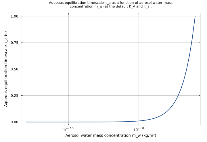
The aqueous equilibration timescale rises linearly with the aerosol water mass concentration (Eq. 12.147). Sweeping m_w over the 1e-9–1e-3 kg/m³ range — from a dilute aerosol-water loading up to a cloud-scale liquid-water content — at the default K_A = 1e-3 kg/m³ and τ_s = 1.0 s traces the line τ_a = (m_w/K_A)·τ_s; τ_a reaches τ_s as m_w approaches K_A.
Time span: 0.0 → 1.0
Swept over: m_w
timescale_vs_equilibrium_constant
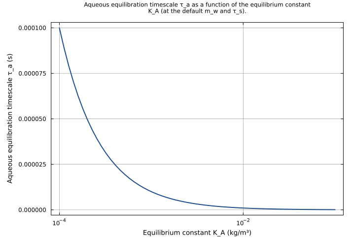
The aqueous equilibration timescale varies inversely with the equilibrium constant (Eq. 12.147). With m_w and τ_s at their defaults, sweeping K_A over the 1e-4–1e-1 kg/m³ range traces the τ_a = (m_w/K_A)·τ_s hyperbola — a larger K_A weakens the Henry’s-law buffering and shortens the equilibration time.
Time span: 0.0 → 1.0
Swept over: K_A
timescale_water_mass_equilibrium_constant_heatmap
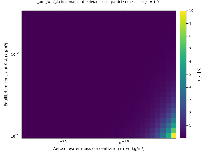
Joint dependence of the aqueous equilibration timescale on the aerosol water mass concentration and the equilibrium constant (Eq. 12.147). The heatmap of τ_a(m_w, K_A) at the default τ_s = 1.0 s shows the timescale rising with the aqueous reservoir m_w and falling with K_A — the buffering-factor m_w/K_A surface.
Time span: 0.0 → 1.0
Swept over: m_w, K_A
Raw .esm
Raw .esm JSON (this component)
{
  "reference": {
    "citation": "Seinfeld, J. H., and Pandis, S. N. (2006). Atmospheric Chemistry and Physics: From Air Pollution to Climate Change, 2nd Edition, John Wiley & Sons, Chapter 12. Aqueous equilibration timescale: Eq. 12.147.",
    "notes": "source_ref: Aerosol.jl@c8c640bb636b22f2425460e9ed5cba50793bfee1:src/timescales.jl:183\n\nUpstream `AqueousEquilibrationTimescale` is an MTK `@component` (no parameterization). It declares three scalar `@parameters` — `m_w` (aerosol water mass concentration, kg/m^3), `K_A` (equilibrium constant, kg/m^3), `τ_s` (solid-particle equilibration timescale, s) — and one scalar `@variable` `τ_a` (aqueous equilibration timescale, s). The single equation is `τ_a ~ (m_w / K_A) * τ_s` — Eq. 12.147 of Seinfeld & Pandis (2006) Ch. 12: the aqueous equilibration timescale is the solid-particle timescale `τ_s` scaled by the dimensionless buffering factor `m_w / K_A`.\n\nτ_s as a parameter: in this isolated component `τ_s` is a free input `@parameter` (default 1.0 s). Physically it is the output of the sibling `SolidEquilibrationTimescale` component (same file, src/timescales.jl:145); the gas-equilibration timescale chain solid → aqueous would be wired by coupling, but each component is migrated standalone, so `τ_s` is carried verbatim as the upstream `@parameter`.\n\nObserved classification: AqueousEquilibrationTimescale has no `D()` time-derivative anywhere — it is a purely-algebraic component. `τ_a` is an algebraic output (`τ_a ~ (m_w/K_A)·τ_s`). After MTK `mtkcompile` / `structural_simplify` the compiled system has zero ODE states and `τ_a` becomes an observed quantity. It is therefore serialized as `type: observed` with an `expression` (not `type: state` with an equation), and the `equations` array is empty, matching the sibling pure-algebraic Aerosol.jl migrations `zsr.esm` and `critical_ssa.esm`.\n\nUnicode identifiers `τ_s` and `τ_a` are kept verbatim from the upstream `@parameters` / `@variables` declarations; the ESM identifier pattern permits unicode and the sibling Aerosol.jl migrations (`zsr.esm`: `α_w`; `kelvin.esm`: `σ`, `ρ_l`) keep Greek symbols, so no ASCII rename is applied.\n\nTests authored from physics: the upstream `timescales.jl` carries no test file (`has_tests: N` in the migration tracker). The inline `tests` block is authored from the closed-form Eq. 12.147 — pinning the exact analytic value of `τ_a = (m_w/K_A)·τ_s` at the upstream default parameterization, at the buffering-factor crossover `m_w = K_A` (where `τ_a = τ_s`), in the strong-buffering regime `m_w ≫ K_A`, and exercising the linear dependence on `m_w` and `τ_s` and the inverse dependence on `K_A`.\n\nNot migrated: `timescales.jl` defines six independent `@component`s — `GasDiffusionTimescale`, `AqueousDiffusionTimescale`, `InterfacialTimescale`, `ReactionTimescale`, `SolidEquilibrationTimescale`, and `AqueousEquilibrationTimescale`. Only `AqueousEquilibrationTimescale` (src/timescales.jl:183) is in scope for this component migration; the other five are separate migration-tracker rows with their own target `.esm` files under `components/aerosol/timescales/`.\n\nTolerance rationale (model-level rel=1e-8): the model is a single closed-form algebraic expression — one division and one multiplication — so float64 evaluation roundoff is at the 1-ULP (~1e-16 relative) level; rel=1e-8 leaves ample headroom. The `zero_water_zero_timescale` test adds a tight per-assertion abs=1e-20 so a stuck-nonzero regression in the `τ_a` product cannot pass on the relative branch."
  },
  "variables": {
    "m_w": {
      "type": "parameter",
      "units": "kg/m^3",
      "default": 1e-08,
      "description": "Aerosol water mass concentration — the mass of liquid water in the aerosol aqueous phase per unit volume of air (Eq. 12.147 term m_w). Sets the size of the aqueous reservoir the gas must fill to reach equilibrium."
    },
    "K_A": {
      "type": "parameter",
      "units": "kg/m^3",
      "default": 0.001,
      "description": "Equilibrium constant (Eq. 12.147 term K_A) — sets the denominator of the dimensionless buffering factor m_w/K_A. A larger K_A weakens the Henry's-law buffering and shortens the aqueous equilibration timescale."
    },
    "τ_s": {
      "type": "parameter",
      "units": "s",
      "default": 1.0,
      "description": "Solid-particle equilibration timescale (Eq. 12.147 term τ_s) — the characteristic time for the gas to equilibrate with solid aerosol particles. A free input parameter here; physically the output of the sibling SolidEquilibrationTimescale component."
    },
    "τ_a": {
      "type": "unknown",
      "units": "s",
      "description": "Aqueous equilibration timescale (Eq. 12.147): τ_a = (m_w/K_A)·τ_s. The characteristic time for the gas to equilibrate with aqueous aerosol particles, equal to the solid-particle timescale τ_s scaled by the dimensionless buffering factor m_w/K_A. A larger aqueous reservoir relative to K_A lengthens the equilibration time."
    }
  },
  "equations": [
    {
      "lhs": "τ_a",
      "rhs": {
        "op": "*",
        "args": [
          {
            "op": "/",
            "args": [
              "m_w",
              "K_A"
            ]
          },
          "τ_s"
        ]
      }
    }
  ],
  "tolerance": {
    "rel": 1e-08
  },
  "tests": [
    {
      "id": "default_parameters",
      "description": "Eq. 12.147 at the upstream default parameterization (m_w = 1e-8 kg/m³, K_A = 1e-3 kg/m³, τ_s = 1.0 s). The buffering factor m_w/K_A = 1e-5 scales the solid-particle timescale to τ_a = (1e-8/1e-3)·1.0 = 1e-5 s — aqueous equilibration is far faster than solid because the aerosol-regime water reservoir is small relative to K_A. The output is algebraic and time-invariant, so the same value is asserted at t = 0 and t = 1.",
      "parameter_overrides": {},
      "time_span": {
        "start": 0.0,
        "end": 1.0
      },
      "assertions": [
        {
          "variable": "τ_a",
          "time": 0.0,
          "expected": 1e-05
        },
        {
          "variable": "τ_a",
          "time": 1.0,
          "expected": 1e-05
        }
      ]
    },
    {
      "id": "buffering_factor_unity",
      "description": "At the buffering-factor crossover m_w = K_A the dimensionless factor m_w/K_A = 1 and the aqueous equilibration timescale equals the solid-particle timescale exactly: τ_a = (1e-3/1e-3)·1.0 = 1.0 s. This is the transition between the fast-aqueous regime (m_w < K_A) and the slow-aqueous regime (m_w > K_A).",
      "parameter_overrides": {
        "m_w": 0.001
      },
      "time_span": {
        "start": 0.0,
        "end": 1.0
      },
      "assertions": [
        {
          "variable": "τ_a",
          "time": 0.0,
          "expected": 1.0
        }
      ]
    },
    {
      "id": "strong_buffering_amplification",
      "description": "In the strong-buffering regime m_w ≫ K_A the aqueous reservoir is large and equilibration is much slower than the solid case. With m_w = 1e-2 kg/m³ (a cloud-scale liquid-water content) and K_A = 1e-3 kg/m³, the buffering factor m_w/K_A = 10 amplifies the solid timescale to τ_a = 10·1.0 = 10.0 s.",
      "parameter_overrides": {
        "m_w": 0.01
      },
      "time_span": {
        "start": 0.0,
        "end": 1.0
      },
      "assertions": [
        {
          "variable": "τ_a",
          "time": 0.0,
          "expected": 10.0
        }
      ]
    },
    {
      "id": "linear_in_water_mass",
      "description": "Eq. 12.147 is linear in the aerosol water mass concentration m_w. Doubling m_w from the 1e-8 default to 2e-8 kg/m³ doubles the aqueous equilibration timescale from 1e-5 to τ_a = (2e-8/1e-3)·1.0 = 2e-5 s — a larger aqueous reservoir takes proportionally longer to fill.",
      "parameter_overrides": {
        "m_w": 2e-08
      },
      "time_span": {
        "start": 0.0,
        "end": 1.0
      },
      "assertions": [
        {
          "variable": "τ_a",
          "time": 0.0,
          "expected": 2e-05
        }
      ]
    },
    {
      "id": "inverse_in_equilibrium_constant",
      "description": "Eq. 12.147 varies inversely with the equilibrium constant K_A. Doubling K_A from the 1e-3 default to 2e-3 kg/m³ halves the aqueous equilibration timescale from 1e-5 to τ_a = (1e-8/2e-3)·1.0 = 5e-6 s — a larger K_A weakens the Henry's-law buffering.",
      "parameter_overrides": {
        "K_A": 0.002
      },
      "time_span": {
        "start": 0.0,
        "end": 1.0
      },
      "assertions": [
        {
          "variable": "τ_a",
          "time": 0.0,
          "expected": 5e-06
        }
      ]
    },
    {
      "id": "linear_in_solid_timescale",
      "description": "Eq. 12.147 scales linearly with the solid-particle equilibration timescale τ_s — the buffering factor m_w/K_A multiplies it directly. Raising τ_s tenfold from 1.0 to 10.0 s raises the aqueous timescale tenfold to τ_a = (1e-8/1e-3)·10.0 = 1e-4 s.",
      "parameter_overrides": {
        "τ_s": 10.0
      },
      "time_span": {
        "start": 0.0,
        "end": 1.0
      },
      "assertions": [
        {
          "variable": "τ_a",
          "time": 0.0,
          "expected": 0.0001
        }
      ]
    },
    {
      "id": "zero_water_zero_timescale",
      "description": "Limiting case: with no aerosol aqueous phase (m_w = 0) the buffering factor m_w/K_A vanishes and τ_a = 0 exactly — there is no aqueous reservoir for the gas to equilibrate with. A tight per-assertion absolute tolerance guards against a stuck-nonzero regression in the τ_a product.",
      "parameter_overrides": {
        "m_w": 0.0
      },
      "time_span": {
        "start": 0.0,
        "end": 1.0
      },
      "assertions": [
        {
          "variable": "τ_a",
          "time": 0.0,
          "expected": 0.0,
          "tolerance": {
            "abs": 1e-20
          }
        }
      ]
    }
  ],
  "analyses": [
    {
      "id": "timescale_vs_water_mass",
      "description": "The aqueous equilibration timescale rises linearly with the aerosol water mass concentration (Eq. 12.147). Sweeping m_w over the 1e-9–1e-3 kg/m³ range — from a dilute aerosol-water loading up to a cloud-scale liquid-water content — at the default K_A = 1e-3 kg/m³ and τ_s = 1.0 s traces the line τ_a = (m_w/K_A)·τ_s; τ_a reaches τ_s as m_w approaches K_A.",
      "parameters": {},
      "time_span": {
        "start": 0.0,
        "end": 1.0
      },
      "parameter_sweep": {
        "type": "cartesian",
        "dimensions": [
          {
            "parameter": "m_w",
            "range": {
              "start": 1e-09,
              "stop": 0.001,
              "count": 60,
              "scale": "log"
            }
          }
        ]
      },
      "plots": [
        {
          "id": "tau_a_vs_m_w",
          "type": "line",
          "description": "Aqueous equilibration timescale τ_a as a function of aerosol water mass concentration m_w (at the default K_A and τ_s).",
          "x": {
            "variable": "m_w",
            "label": "Aerosol water mass concentration m_w (kg/m³)"
          },
          "y": {
            "variable": "τ_a",
            "label": "Aqueous equilibration timescale τ_a (s)"
          }
        }
      ]
    },
    {
      "id": "timescale_vs_equilibrium_constant",
      "description": "The aqueous equilibration timescale varies inversely with the equilibrium constant (Eq. 12.147). With m_w and τ_s at their defaults, sweeping K_A over the 1e-4–1e-1 kg/m³ range traces the τ_a = (m_w/K_A)·τ_s hyperbola — a larger K_A weakens the Henry's-law buffering and shortens the equilibration time.",
      "parameters": {},
      "time_span": {
        "start": 0.0,
        "end": 1.0
      },
      "parameter_sweep": {
        "type": "cartesian",
        "dimensions": [
          {
            "parameter": "K_A",
            "range": {
              "start": 0.0001,
              "stop": 0.1,
              "count": 60,
              "scale": "log"
            }
          }
        ]
      },
      "plots": [
        {
          "id": "tau_a_vs_K_A",
          "type": "line",
          "description": "Aqueous equilibration timescale τ_a as a function of the equilibrium constant K_A (at the default m_w and τ_s).",
          "x": {
            "variable": "K_A",
            "label": "Equilibrium constant K_A (kg/m³)"
          },
          "y": {
            "variable": "τ_a",
            "label": "Aqueous equilibration timescale τ_a (s)"
          }
        }
      ]
    },
    {
      "id": "timescale_water_mass_equilibrium_constant_heatmap",
      "description": "Joint dependence of the aqueous equilibration timescale on the aerosol water mass concentration and the equilibrium constant (Eq. 12.147). The heatmap of τ_a(m_w, K_A) at the default τ_s = 1.0 s shows the timescale rising with the aqueous reservoir m_w and falling with K_A — the buffering-factor m_w/K_A surface.",
      "parameters": {},
      "time_span": {
        "start": 0.0,
        "end": 1.0
      },
      "parameter_sweep": {
        "type": "cartesian",
        "dimensions": [
          {
            "parameter": "m_w",
            "range": {
              "start": 1e-09,
              "stop": 0.001,
              "count": 30,
              "scale": "log"
            }
          },
          {
            "parameter": "K_A",
            "range": {
              "start": 0.0001,
              "stop": 0.1,
              "count": 25,
              "scale": "log"
            }
          }
        ]
      },
      "plots": [
        {
          "id": "tau_a_m_w_K_A_heatmap",
          "type": "heatmap",
          "description": "τ_a(m_w, K_A) heatmap at the default solid-particle timescale τ_s = 1.0 s.",
          "x": {
            "variable": "m_w",
            "label": "Aerosol water mass concentration m_w (kg/m³)"
          },
          "y": {
            "variable": "K_A",
            "label": "Equilibrium constant K_A (kg/m³)"
          },
          "value": {
            "variable": "τ_a",
            "reduce": "final"
          }
        }
      ]
    }
  ]
}