AerosolDistribution
ModelingToolkit implementation of a multi-modal lognormal atmospheric aerosol size distribution, from Seinfeld & Pandis (2006), Atmospheric Chemistry and Physics, 2nd ed., Chapter 8 ("Properties of the Atmospheric Aerosol"). The model represents the aerosol number, surface-area and volume distributions as a sum of three lognormal modes (Eq. 8.54), and reports the total number/surface/volume concentrations, the mode-1 Hatch-Choate diameters, and the vertical aerosol mass profile (Eq. 8.55). Migrated from Aerosol.jl AerosolDistribution. Purely algebraic: ten observed outputs, no differential states, an empty equations array. The upstream length-n_modes array parameters are scalarized at the default and documented n_modes = 3; default mode parameters are the Urban distribution of Table 8.3.
Description
ModelingToolkit implementation of a multi-modal lognormal atmospheric aerosol size distribution, from Seinfeld & Pandis (2006), Atmospheric Chemistry and Physics, 2nd ed., Chapter 8 (“Properties of the Atmospheric Aerosol”). The model represents the aerosol number, surface-area and volume distributions as a sum of three lognormal modes (Eq. 8.54), and reports the total number/surface/volume concentrations, the mode-1 Hatch-Choate diameters, and the vertical aerosol mass profile (Eq. 8.55). Migrated from Aerosol.jl AerosolDistribution. Purely algebraic: ten observed outputs, no differential states, an empty equations array. The upstream length-n_modes array parameters are scalarized at the default and documented n_modes = 3; default mode parameters are the Urban distribution of Table 8.3.
Reference
Seinfeld, J. H., and Pandis, S. N. (2006). Atmospheric Chemistry and Physics: From Air Pollution to Climate Change, 2nd Edition, John Wiley & Sons, Chapter 8, “Properties of the Atmospheric Aerosol”. Multi-modal lognormal size distribution: Eq. 8.54 (number), 8.49/8.50 (surface area), 8.52/8.53 (volume); Hatch-Choate diameters Eq. 8.44/8.50/8.53; total moments Eq. 8.41 with Eq. 8.5/8.7; vertical mass profile Eq. 8.55; default mode parameters from the Urban entry of Table 8.3.
_source_ref: Aerosol.jl@c8c640bb636b22f2425460e9ed5cba50793bfee1:src/size_distribution.jl:25
Upstream AerosolDistribution(n_modes=3; ...) is an MTK @component describing a multi-modal lognormal aerosol size distribution (Seinfeld & Pandis 2006, Chapter 8). It carries two @constants (pi_c = pi, ln10 = log(10)), the length-n_modes array @parameters N / D_g / logsigma plus the scalar @parameters D_p, rho_p, z, H_p, and ten time-indexed @variables (n_N_o, n_S_o, n_V_o, N_t, S_t, V_t, D_s, D_v, D_bar, M_z), each defined by one algebraic lhs ~ rhs equation. There is no D(.) time derivative anywhere.
Observability classification: observed-form. Every one of the ten equation right-hand sides references only upstream @parameters and @constants — there is no upstream input @variable (connected input) on any RHS. Per the purely-algebraic migration rule, a component whose equation RHSs are parameter-only migrates in observed-form: each of the ten outputs is encoded as type: observed carrying its defining relation in the expression field, and the equations array is empty. This matches sibling parameter-only algebraic migrations (aqueous_eq.esm, gas_diffusion.esm, critical_ssa.esm).
Array scalarization: the upstream N, D_g and logsigma are length-n_modes array @parameters. The component’s default and documented configuration is n_modes = 3 (a three-mode lognormal); the seven predefined distributions in the same source file (Urban/Marine/Rural/…) are all three-mode. The .esm array-variable path emits getindex nodes (tracked upstream as gt-p3ep), so this migration scalarizes the three modes into nine scalar parameters N_1..N_3, D_g_1..D_g_3, logsigma_1..logsigma_3 and unrolls each sum(... for i in 1:n_modes) into an explicit three-term sum. This is the faithful migration of the default three-mode component; the non-default n_modes are not represented.
Constant handling: pi_c and ln10 are upstream @constants. The ESS schema has no constant variable type, so each migrates as a type: parameter with a fixed evaluated numeric default (pi_c = 3.141592653589793, ln10 = 2.302585092994046); the symbols are kept in the expressions. ln10 carries the conversion from the log10-based logsigma to natural-log form: ln(sigma_g) = logsigma * ln10, which is why the moment/Hatch-Choate factors read exp(k*(logsigma*ln10)^2).
Pruned parameter: the upstream @parameter rho_p (particle density, default 1500 kg/m^3) appears in none of the ten equations and is therefore not collected by System(eqs, t). It is omitted from this migration per the unused-parameter rule — the model computes number, surface-area and volume distributions and a dimensionless vertical mass ratio, none of which require a density.
Defaults: the upstream base AerosolDistribution(3) declares N, D_g, logsigma and D_p with no defaults (defaults are supplied only by the predefined wrappers such as UrbanAerosol). The docstring states “Default parameter values correspond to the ‘Urban’ distribution from Table 8.3”, so this migration adopts the Urban Table 8.3 values as the defaults of N_1..3, D_g_1..3 and logsigma_1..3 (N converted cm^-3 -> m^-3 by x1e6, D_g um -> m by x1e-6). D_p defaults to 1.0e-7 m (0.1 um), the diameter the upstream test suite evaluates the distributions at; z = 0 and H_p = 1000 m are the upstream scalar defaults.
Tests: the nine inline tests below are translated from the upstream test suite test/size_distribution_test.jl. The single-mode upstream cases (AerosolDistribution(1)) are reproduced on the fixed three-mode .esm by zeroing the mode-2 and mode-3 number concentrations (N_2 = N_3 = 0), which removes their contribution to every sum; D_s, D_v and D_bar depend on mode 1 only by construction. Coverage spans all ten outputs, the three Table 8.3 presets (Urban/Marine/Remote continental), the lognormal peak and one-sigma points, log-space symmetry, the Hatch-Choate diameter ordering, the moment forms and the vertical mass profile.
Tolerance rationale (model-level rel=1e-9): the component is purely algebraic with no ODE integration. Each output is a finite composition of +, , /, ^, sqrt, exp and log10 in float64 (round-off ~1e-16 relative); rel=1e-9 leaves seven orders of magnitude of headroom and absorbs any associativity difference in the n-ary sums and products. The pinned expected values are the exact textbook-formula results, cross-checked at generation time against the closed-form Seinfeld & Pandis relations the upstream test suite asserts (peak = N/(sqrt(2pi)*logsigma), the Hatch-Choate ratio D_v/D_s = exp(ln^2 sigma), the moment forms, M_z = exp(-z/H_p)).
Units: descriptive only; the ESS runners do no dimensional analysis. Units are copied from the upstream unit metadata verbatim (n_S_o / S_t in m^-1, n_V_o / V_t / M_z dimensionless)._
Parameters
| Name | Units | Default | Description |
|---|---|---|---|
π_c | 1 | 3.141592653589793 | Pi (mathematical constant). Upstream MTK @constants entry pi_c = pi; the ESS schema has no constant variable type, so it migrates as a fixed-default parameter with the evaluated numeric value. |
ln10 | 1 | 2.302585092994046 | Natural logarithm of 10. Upstream MTK @constants entry ln10 = log(10.0); migrated as a fixed-default parameter. Converts the log10-based geometric standard deviations logsigma to natural-log form, ln(sigma_g) = logsigma * ln10. |
N_1 | m^-3 | 99300000000.0 | Total number concentration of mode 1 (nucleation). Upstream array @parameter N[1]. Default: Urban distribution, Seinfeld & Pandis (2006) Table 8.3. |
N_2 | m^-3 | 1110000000.0 | Total number concentration of mode 2 (Aitken). Upstream array @parameter N[2]. Default: Urban distribution, Seinfeld & Pandis (2006) Table 8.3. |
N_3 | m^-3 | 36400000000.0 | Total number concentration of mode 3 (accumulation). Upstream array @parameter N[3]. Default: Urban distribution, Seinfeld & Pandis (2006) Table 8.3. |
D_g_1 | m | 1.3e-08 | Geometric median diameter of mode 1 (nucleation). Upstream array @parameter D_g[1]. Default: Urban distribution, Seinfeld & Pandis (2006) Table 8.3. |
D_g_2 | m | 1.4e-08 | Geometric median diameter of mode 2 (Aitken). Upstream array @parameter D_g[2]. Default: Urban distribution, Seinfeld & Pandis (2006) Table 8.3. |
D_g_3 | m | 5e-08 | Geometric median diameter of mode 3 (accumulation). Upstream array @parameter D_g[3]. Default: Urban distribution, Seinfeld & Pandis (2006) Table 8.3. |
logσ_1 | 1 | 0.245 | Log10 of the geometric standard deviation of mode 1 (nucleation) (dimensionless). Upstream array @parameter logsigma[1]. Default: Urban distribution, Seinfeld & Pandis (2006) Table 8.3. |
logσ_2 | 1 | 0.666 | Log10 of the geometric standard deviation of mode 2 (Aitken) (dimensionless). Upstream array @parameter logsigma[2]. Default: Urban distribution, Seinfeld & Pandis (2006) Table 8.3. |
logσ_3 | 1 | 0.337 | Log10 of the geometric standard deviation of mode 3 (accumulation) (dimensionless). Upstream array @parameter logsigma[3]. Default: Urban distribution, Seinfeld & Pandis (2006) Table 8.3. |
D_p | m | 1e-07 | Particle diameter at which the number, surface-area and volume distribution densities n_N_o/n_S_o/n_V_o are evaluated. The upstream base AerosolDistribution declares D_p with no default; 1.0e-7 m (0.1 um) is adopted here — the diameter the upstream test suite evaluates the distributions at, in the accumulation-mode range. |
z | m | 0.0 | Altitude above the surface, used by the vertical mass profile M_z. Default 0 m (surface). Upstream @parameter z = 0.0. |
H_p | m | 1000.0 | Aerosol mass scale height in the vertical profile M_z = exp(-z/H_p). Default 1000 m. Upstream @parameter H_p = 1000.0. |
Observed
| Name | Units | Default | Description |
|---|---|---|---|
n_N_o | m^-3 | Number distribution density dN/d(log D_p) at the evaluation diameter D_p — the sum of n_modes lognormal modes (Seinfeld & Pandis 2006, Eq. 8.54). | |
n_S_o | m^-1 | Surface-area distribution density dS/d(log D_p) at D_p (Seinfeld & Pandis 2006, Eq. 8.49/8.50). | |
n_V_o | 1 | Volume distribution density dV/d(log D_p) at D_p (Seinfeld & Pandis 2006, Eq. 8.52/8.53). | |
N_t | m^-3 | Total number concentration — the sum of the per-mode number concentrations N_i. | |
S_t | m^-1 | Total surface-area concentration — Seinfeld & Pandis (2006) Eq. 8.5 evaluated with the k=2 lognormal moment Eq. 8.41. | |
V_t | 1 | Total volume concentration — Seinfeld & Pandis (2006) Eq. 8.7 evaluated with the k=3 lognormal moment Eq. 8.41. | |
D_s | m | Surface-area median diameter of mode 1 — the Hatch-Choate relation D_s = D_g * exp(2*ln^2 sigma_g) (Seinfeld & Pandis 2006, Eq. 8.50). | |
D_v | m | Volume median diameter of mode 1 — the Hatch-Choate relation D_v = D_g * exp(3*ln^2 sigma_g) (Seinfeld & Pandis 2006, Eq. 8.53). | |
D_bar | m | Mean diameter of mode 1 — the Hatch-Choate relation D_bar = D_g * exp(0.5*ln^2 sigma_g) (Seinfeld & Pandis 2006, Eq. 8.44). | |
M_z | 1 | Vertical aerosol mass profile ratio M(z)/M(0) = exp(-z/H_p) (Seinfeld & Pandis 2006, Eq. 8.55), dimensionless. |
Observed expressions
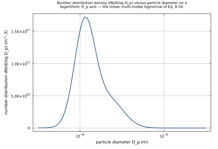
$$ n_{N\,o} = \frac{N_{1}}{\sqrt{2 \cdot π_{c}} \cdot logσ_{1}} \cdot e^{\frac{-\log_{10}\left(\frac{D_{p}}{D_{g\,1}}\right)^{2}}{2 \cdot logσ_{1}^{2}}} + \frac{N_{2}}{\sqrt{2 \cdot π_{c}} \cdot logσ_{2}} \cdot e^{\frac{-\log_{10}\left(\frac{D_{p}}{D_{g\,2}}\right)^{2}}{2 \cdot logσ_{2}^{2}}} + \frac{N_{3}}{\sqrt{2 \cdot π_{c}} \cdot logσ_{3}} \cdot e^{\frac{-\log_{10}\left(\frac{D_{p}}{D_{g\,3}}\right)^{2}}{2 \cdot logσ_{3}^{2}}} $$Number distribution density dN/d(log D_p) at the evaluation diameter D_p — the sum of n_modes lognormal modes (Seinfeld & Pandis 2006, Eq. 8.54).
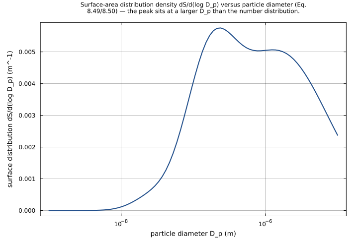
$$ n_{S\,o} = \frac{π_{c} \cdot N_{1} \cdot \left(D_{g\,1} \cdot e^{2 \cdot \left(logσ_{1} \cdot ln10\right)^{2}}\right)^{2}}{\sqrt{2 \cdot π_{c}} \cdot logσ_{1}} \cdot e^{\frac{-\log_{10}\left(\frac{D_{p}}{D_{g\,1} \cdot e^{2 \cdot \left(logσ_{1} \cdot ln10\right)^{2}}}\right)^{2}}{2 \cdot logσ_{1}^{2}}} + \frac{π_{c} \cdot N_{2} \cdot \left(D_{g\,2} \cdot e^{2 \cdot \left(logσ_{2} \cdot ln10\right)^{2}}\right)^{2}}{\sqrt{2 \cdot π_{c}} \cdot logσ_{2}} \cdot e^{\frac{-\log_{10}\left(\frac{D_{p}}{D_{g\,2} \cdot e^{2 \cdot \left(logσ_{2} \cdot ln10\right)^{2}}}\right)^{2}}{2 \cdot logσ_{2}^{2}}} + \frac{π_{c} \cdot N_{3} \cdot \left(D_{g\,3} \cdot e^{2 \cdot \left(logσ_{3} \cdot ln10\right)^{2}}\right)^{2}}{\sqrt{2 \cdot π_{c}} \cdot logσ_{3}} \cdot e^{\frac{-\log_{10}\left(\frac{D_{p}}{D_{g\,3} \cdot e^{2 \cdot \left(logσ_{3} \cdot ln10\right)^{2}}}\right)^{2}}{2 \cdot logσ_{3}^{2}}} $$Surface-area distribution density dS/d(log D_p) at D_p (Seinfeld & Pandis 2006, Eq. 8.49/8.50).
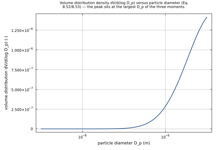
$$ n_{V\,o} = \frac{\frac{π_{c}}{6} \cdot N_{1} \cdot \left(D_{g\,1} \cdot e^{3 \cdot \left(logσ_{1} \cdot ln10\right)^{2}}\right)^{3}}{\sqrt{2 \cdot π_{c}} \cdot logσ_{1}} \cdot e^{\frac{-\log_{10}\left(\frac{D_{p}}{D_{g\,1} \cdot e^{3 \cdot \left(logσ_{1} \cdot ln10\right)^{2}}}\right)^{2}}{2 \cdot logσ_{1}^{2}}} + \frac{\frac{π_{c}}{6} \cdot N_{2} \cdot \left(D_{g\,2} \cdot e^{3 \cdot \left(logσ_{2} \cdot ln10\right)^{2}}\right)^{3}}{\sqrt{2 \cdot π_{c}} \cdot logσ_{2}} \cdot e^{\frac{-\log_{10}\left(\frac{D_{p}}{D_{g\,2} \cdot e^{3 \cdot \left(logσ_{2} \cdot ln10\right)^{2}}}\right)^{2}}{2 \cdot logσ_{2}^{2}}} + \frac{\frac{π_{c}}{6} \cdot N_{3} \cdot \left(D_{g\,3} \cdot e^{3 \cdot \left(logσ_{3} \cdot ln10\right)^{2}}\right)^{3}}{\sqrt{2 \cdot π_{c}} \cdot logσ_{3}} \cdot e^{\frac{-\log_{10}\left(\frac{D_{p}}{D_{g\,3} \cdot e^{3 \cdot \left(logσ_{3} \cdot ln10\right)^{2}}}\right)^{2}}{2 \cdot logσ_{3}^{2}}} $$Volume distribution density dV/d(log D_p) at D_p (Seinfeld & Pandis 2006, Eq. 8.52/8.53).
$$ N_{t} = N_{1} + N_{2} + N_{3} $$Total number concentration — the sum of the per-mode number concentrations N_i.
$$ S_{t} = π_{c} \cdot N_{1} \cdot D_{g\,1}^{2} \cdot e^{2 \cdot \left(logσ_{1} \cdot ln10\right)^{2}} + π_{c} \cdot N_{2} \cdot D_{g\,2}^{2} \cdot e^{2 \cdot \left(logσ_{2} \cdot ln10\right)^{2}} + π_{c} \cdot N_{3} \cdot D_{g\,3}^{2} \cdot e^{2 \cdot \left(logσ_{3} \cdot ln10\right)^{2}} $$Total surface-area concentration — Seinfeld & Pandis (2006) Eq. 8.5 evaluated with the k=2 lognormal moment Eq. 8.41.
$$ V_{t} = \frac{π_{c}}{6} \cdot N_{1} \cdot D_{g\,1}^{3} \cdot e^{4.5 \cdot \left(logσ_{1} \cdot ln10\right)^{2}} + \frac{π_{c}}{6} \cdot N_{2} \cdot D_{g\,2}^{3} \cdot e^{4.5 \cdot \left(logσ_{2} \cdot ln10\right)^{2}} + \frac{π_{c}}{6} \cdot N_{3} \cdot D_{g\,3}^{3} \cdot e^{4.5 \cdot \left(logσ_{3} \cdot ln10\right)^{2}} $$Total volume concentration — Seinfeld & Pandis (2006) Eq. 8.7 evaluated with the k=3 lognormal moment Eq. 8.41.
$$ D_{s} = D_{g\,1} \cdot e^{2 \cdot \left(logσ_{1} \cdot ln10\right)^{2}} $$Surface-area median diameter of mode 1 — the Hatch-Choate relation D_s = D_g * exp(2*ln^2 sigma_g) (Seinfeld & Pandis 2006, Eq. 8.50).
$$ D_{v} = D_{g\,1} \cdot e^{3 \cdot \left(logσ_{1} \cdot ln10\right)^{2}} $$Volume median diameter of mode 1 — the Hatch-Choate relation D_v = D_g * exp(3*ln^2 sigma_g) (Seinfeld & Pandis 2006, Eq. 8.53).
$$ D_{bar} = D_{g\,1} \cdot e^{0.5 \cdot \left(logσ_{1} \cdot ln10\right)^{2}} $$Mean diameter of mode 1 — the Hatch-Choate relation D_bar = D_g * exp(0.5*ln^2 sigma_g) (Seinfeld & Pandis 2006, Eq. 8.44).
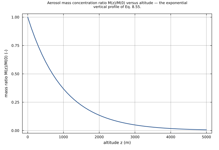
$$ M_{z} = e^{-\frac{z}{H_{p}}} $$Vertical aerosol mass profile ratio M(z)/M(0) = exp(-z/H_p) (Seinfeld & Pandis 2006, Eq. 8.55), dimensionless.
Analyses
aerosol_size_distribution_curves
The canonical Seinfeld & Pandis Chapter 8 figure: the Urban multi-modal lognormal aerosol size distribution. Sweeps the evaluation diameter D_p logarithmically across the full atmospheric aerosol range (1 nm to 10 um) and plots the number (n_N_o, Eq. 8.54), surface-area (n_S_o, Eq. 8.49/8.50) and volume (n_V_o, Eq. 8.52/8.53) distribution densities. The characteristic shift of the distribution peak toward larger diameters going from number to surface to volume is the headline result of this section.
Time span: 0.0 → 1.0
Swept over: D_p
vertical_mass_profile
Vertical aerosol mass profile of Seinfeld & Pandis Eq. 8.55. Sweeps altitude z from the surface to 5 km and plots the mass concentration ratio M_z = M(z)/M(0) = exp(-z/H_p) with the default scale height H_p = 1000 m. The profile decays exponentially, reaching 1/e of the surface value at z = H_p.
Time span: 0.0 → 1.0
Swept over: z
Raw .esm
Raw .esm JSON (this component)
{
"reference": {
"citation": "Seinfeld, J. H., and Pandis, S. N. (2006). Atmospheric Chemistry and Physics: From Air Pollution to Climate Change, 2nd Edition, John Wiley & Sons, Chapter 8, \"Properties of the Atmospheric Aerosol\". Multi-modal lognormal size distribution: Eq. 8.54 (number), 8.49/8.50 (surface area), 8.52/8.53 (volume); Hatch-Choate diameters Eq. 8.44/8.50/8.53; total moments Eq. 8.41 with Eq. 8.5/8.7; vertical mass profile Eq. 8.55; default mode parameters from the Urban entry of Table 8.3.",
"notes": "source_ref: Aerosol.jl@c8c640bb636b22f2425460e9ed5cba50793bfee1:src/size_distribution.jl:25\n\nUpstream `AerosolDistribution(n_modes=3; ...)` is an MTK `@component` describing a multi-modal lognormal aerosol size distribution (Seinfeld & Pandis 2006, Chapter 8). It carries two `@constants` (pi_c = pi, ln10 = log(10)), the length-`n_modes` array `@parameters` N / D_g / logsigma plus the scalar `@parameters` D_p, rho_p, z, H_p, and ten time-indexed `@variables` (n_N_o, n_S_o, n_V_o, N_t, S_t, V_t, D_s, D_v, D_bar, M_z), each defined by one algebraic `lhs ~ rhs` equation. There is no `D(.)` time derivative anywhere.\n\nObservability classification: observed-form. Every one of the ten equation right-hand sides references only upstream `@parameters` and `@constants` — there is no upstream input `@variable` (connected input) on any RHS. Per the purely-algebraic migration rule, a component whose equation RHSs are parameter-only migrates in observed-form: each of the ten outputs is encoded as `type: observed` carrying its defining relation in the `expression` field, and the `equations` array is empty. This matches sibling parameter-only algebraic migrations (aqueous_eq.esm, gas_diffusion.esm, critical_ssa.esm).\n\nArray scalarization: the upstream N, D_g and logsigma are length-`n_modes` array `@parameters`. The component's default and documented configuration is `n_modes = 3` (a three-mode lognormal); the seven predefined distributions in the same source file (Urban/Marine/Rural/...) are all three-mode. The `.esm` array-variable path emits `getindex` nodes (tracked upstream as gt-p3ep), so this migration scalarizes the three modes into nine scalar parameters N_1..N_3, D_g_1..D_g_3, logsigma_1..logsigma_3 and unrolls each `sum(... for i in 1:n_modes)` into an explicit three-term sum. This is the faithful migration of the default three-mode component; the non-default n_modes are not represented.\n\nConstant handling: pi_c and ln10 are upstream `@constants`. The ESS schema has no constant variable type, so each migrates as a `type: parameter` with a fixed evaluated numeric default (pi_c = 3.141592653589793, ln10 = 2.302585092994046); the symbols are kept in the expressions. ln10 carries the conversion from the log10-based logsigma to natural-log form: ln(sigma_g) = logsigma * ln10, which is why the moment/Hatch-Choate factors read exp(k*(logsigma*ln10)^2).\n\nPruned parameter: the upstream `@parameter rho_p` (particle density, default 1500 kg/m^3) appears in none of the ten equations and is therefore not collected by `System(eqs, t)`. It is omitted from this migration per the unused-parameter rule — the model computes number, surface-area and volume distributions and a dimensionless vertical mass ratio, none of which require a density.\n\nDefaults: the upstream base `AerosolDistribution(3)` declares N, D_g, logsigma and D_p with no defaults (defaults are supplied only by the predefined wrappers such as `UrbanAerosol`). The docstring states \"Default parameter values correspond to the 'Urban' distribution from Table 8.3\", so this migration adopts the Urban Table 8.3 values as the defaults of N_1..3, D_g_1..3 and logsigma_1..3 (N converted cm^-3 -> m^-3 by x1e6, D_g um -> m by x1e-6). D_p defaults to 1.0e-7 m (0.1 um), the diameter the upstream test suite evaluates the distributions at; z = 0 and H_p = 1000 m are the upstream scalar defaults.\n\nTests: the nine inline tests below are translated from the upstream test suite test/size_distribution_test.jl. The single-mode upstream cases (AerosolDistribution(1)) are reproduced on the fixed three-mode .esm by zeroing the mode-2 and mode-3 number concentrations (N_2 = N_3 = 0), which removes their contribution to every sum; D_s, D_v and D_bar depend on mode 1 only by construction. Coverage spans all ten outputs, the three Table 8.3 presets (Urban/Marine/Remote continental), the lognormal peak and one-sigma points, log-space symmetry, the Hatch-Choate diameter ordering, the moment forms and the vertical mass profile.\n\nTolerance rationale (model-level rel=1e-9): the component is purely algebraic with no ODE integration. Each output is a finite composition of +, *, /, ^, sqrt, exp and log10 in float64 (round-off ~1e-16 relative); rel=1e-9 leaves seven orders of magnitude of headroom and absorbs any associativity difference in the n-ary sums and products. The pinned expected values are the exact textbook-formula results, cross-checked at generation time against the closed-form Seinfeld & Pandis relations the upstream test suite asserts (peak = N/(sqrt(2*pi)*logsigma), the Hatch-Choate ratio D_v/D_s = exp(ln^2 sigma), the moment forms, M_z = exp(-z/H_p)).\n\nUnits: descriptive only; the ESS runners do no dimensional analysis. Units are copied from the upstream `unit` metadata verbatim (n_S_o / S_t in m^-1, n_V_o / V_t / M_z dimensionless)."
},
"tolerance": {
"rel": 1e-09
},
"variables": {
"π_c": {
"type": "parameter",
"units": "1",
"default": 3.141592653589793,
"description": "Pi (mathematical constant). Upstream MTK @constants entry pi_c = pi; the ESS schema has no constant variable type, so it migrates as a fixed-default parameter with the evaluated numeric value."
},
"ln10": {
"type": "parameter",
"units": "1",
"default": 2.302585092994046,
"description": "Natural logarithm of 10. Upstream MTK @constants entry ln10 = log(10.0); migrated as a fixed-default parameter. Converts the log10-based geometric standard deviations logsigma to natural-log form, ln(sigma_g) = logsigma * ln10."
},
"N_1": {
"type": "parameter",
"units": "m^-3",
"default": 99300000000.0,
"description": "Total number concentration of mode 1 (nucleation). Upstream array @parameter N[1]. Default: Urban distribution, Seinfeld & Pandis (2006) Table 8.3."
},
"N_2": {
"type": "parameter",
"units": "m^-3",
"default": 1110000000.0,
"description": "Total number concentration of mode 2 (Aitken). Upstream array @parameter N[2]. Default: Urban distribution, Seinfeld & Pandis (2006) Table 8.3."
},
"N_3": {
"type": "parameter",
"units": "m^-3",
"default": 36400000000.0,
"description": "Total number concentration of mode 3 (accumulation). Upstream array @parameter N[3]. Default: Urban distribution, Seinfeld & Pandis (2006) Table 8.3."
},
"D_g_1": {
"type": "parameter",
"units": "m",
"default": 1.3e-08,
"description": "Geometric median diameter of mode 1 (nucleation). Upstream array @parameter D_g[1]. Default: Urban distribution, Seinfeld & Pandis (2006) Table 8.3."
},
"D_g_2": {
"type": "parameter",
"units": "m",
"default": 1.4e-08,
"description": "Geometric median diameter of mode 2 (Aitken). Upstream array @parameter D_g[2]. Default: Urban distribution, Seinfeld & Pandis (2006) Table 8.3."
},
"D_g_3": {
"type": "parameter",
"units": "m",
"default": 5e-08,
"description": "Geometric median diameter of mode 3 (accumulation). Upstream array @parameter D_g[3]. Default: Urban distribution, Seinfeld & Pandis (2006) Table 8.3."
},
"logσ_1": {
"type": "parameter",
"units": "1",
"default": 0.245,
"description": "Log10 of the geometric standard deviation of mode 1 (nucleation) (dimensionless). Upstream array @parameter logsigma[1]. Default: Urban distribution, Seinfeld & Pandis (2006) Table 8.3."
},
"logσ_2": {
"type": "parameter",
"units": "1",
"default": 0.666,
"description": "Log10 of the geometric standard deviation of mode 2 (Aitken) (dimensionless). Upstream array @parameter logsigma[2]. Default: Urban distribution, Seinfeld & Pandis (2006) Table 8.3."
},
"logσ_3": {
"type": "parameter",
"units": "1",
"default": 0.337,
"description": "Log10 of the geometric standard deviation of mode 3 (accumulation) (dimensionless). Upstream array @parameter logsigma[3]. Default: Urban distribution, Seinfeld & Pandis (2006) Table 8.3."
},
"D_p": {
"type": "parameter",
"units": "m",
"default": 1e-07,
"description": "Particle diameter at which the number, surface-area and volume distribution densities n_N_o/n_S_o/n_V_o are evaluated. The upstream base AerosolDistribution declares D_p with no default; 1.0e-7 m (0.1 um) is adopted here — the diameter the upstream test suite evaluates the distributions at, in the accumulation-mode range."
},
"z": {
"type": "parameter",
"units": "m",
"default": 0.0,
"description": "Altitude above the surface, used by the vertical mass profile M_z. Default 0 m (surface). Upstream @parameter z = 0.0."
},
"H_p": {
"type": "parameter",
"units": "m",
"default": 1000.0,
"description": "Aerosol mass scale height in the vertical profile M_z = exp(-z/H_p). Default 1000 m. Upstream @parameter H_p = 1000.0."
},
"n_N_o": {
"type": "unknown",
"units": "m^-3",
"description": "Number distribution density dN/d(log D_p) at the evaluation diameter D_p — the sum of n_modes lognormal modes (Seinfeld & Pandis 2006, Eq. 8.54)."
},
"n_S_o": {
"type": "unknown",
"units": "m^-1",
"description": "Surface-area distribution density dS/d(log D_p) at D_p (Seinfeld & Pandis 2006, Eq. 8.49/8.50)."
},
"n_V_o": {
"type": "unknown",
"units": "1",
"description": "Volume distribution density dV/d(log D_p) at D_p (Seinfeld & Pandis 2006, Eq. 8.52/8.53)."
},
"N_t": {
"type": "unknown",
"units": "m^-3",
"description": "Total number concentration — the sum of the per-mode number concentrations N_i."
},
"S_t": {
"type": "unknown",
"units": "m^-1",
"description": "Total surface-area concentration — Seinfeld & Pandis (2006) Eq. 8.5 evaluated with the k=2 lognormal moment Eq. 8.41."
},
"V_t": {
"type": "unknown",
"units": "1",
"description": "Total volume concentration — Seinfeld & Pandis (2006) Eq. 8.7 evaluated with the k=3 lognormal moment Eq. 8.41."
},
"D_s": {
"type": "unknown",
"units": "m",
"description": "Surface-area median diameter of mode 1 — the Hatch-Choate relation D_s = D_g * exp(2*ln^2 sigma_g) (Seinfeld & Pandis 2006, Eq. 8.50)."
},
"D_v": {
"type": "unknown",
"units": "m",
"description": "Volume median diameter of mode 1 — the Hatch-Choate relation D_v = D_g * exp(3*ln^2 sigma_g) (Seinfeld & Pandis 2006, Eq. 8.53)."
},
"D_bar": {
"type": "unknown",
"units": "m",
"description": "Mean diameter of mode 1 — the Hatch-Choate relation D_bar = D_g * exp(0.5*ln^2 sigma_g) (Seinfeld & Pandis 2006, Eq. 8.44)."
},
"M_z": {
"type": "unknown",
"units": "1",
"description": "Vertical aerosol mass profile ratio M(z)/M(0) = exp(-z/H_p) (Seinfeld & Pandis 2006, Eq. 8.55), dimensionless."
}
},
"equations": [
{
"lhs": "n_N_o",
"rhs": {
"op": "+",
"args": [
{
"op": "*",
"args": [
{
"op": "/",
"args": [
"N_1",
{
"op": "*",
"args": [
{
"op": "sqrt",
"args": [
{
"op": "*",
"args": [
2,
"π_c"
]
}
]
},
"logσ_1"
]
}
]
},
{
"op": "exp",
"args": [
{
"op": "/",
"args": [
{
"op": "-",
"args": [
{
"op": "^",
"args": [
{
"op": "log10",
"args": [
{
"op": "/",
"args": [
"D_p",
"D_g_1"
]
}
]
},
2
]
}
]
},
{
"op": "*",
"args": [
2,
{
"op": "^",
"args": [
"logσ_1",
2
]
}
]
}
]
}
]
}
]
},
{
"op": "*",
"args": [
{
"op": "/",
"args": [
"N_2",
{
"op": "*",
"args": [
{
"op": "sqrt",
"args": [
{
"op": "*",
"args": [
2,
"π_c"
]
}
]
},
"logσ_2"
]
}
]
},
{
"op": "exp",
"args": [
{
"op": "/",
"args": [
{
"op": "-",
"args": [
{
"op": "^",
"args": [
{
"op": "log10",
"args": [
{
"op": "/",
"args": [
"D_p",
"D_g_2"
]
}
]
},
2
]
}
]
},
{
"op": "*",
"args": [
2,
{
"op": "^",
"args": [
"logσ_2",
2
]
}
]
}
]
}
]
}
]
},
{
"op": "*",
"args": [
{
"op": "/",
"args": [
"N_3",
{
"op": "*",
"args": [
{
"op": "sqrt",
"args": [
{
"op": "*",
"args": [
2,
"π_c"
]
}
]
},
"logσ_3"
]
}
]
},
{
"op": "exp",
"args": [
{
"op": "/",
"args": [
{
"op": "-",
"args": [
{
"op": "^",
"args": [
{
"op": "log10",
"args": [
{
"op": "/",
"args": [
"D_p",
"D_g_3"
]
}
]
},
2
]
}
]
},
{
"op": "*",
"args": [
2,
{
"op": "^",
"args": [
"logσ_3",
2
]
}
]
}
]
}
]
}
]
}
]
}
},
{
"lhs": "n_S_o",
"rhs": {
"op": "+",
"args": [
{
"op": "*",
"args": [
{
"op": "/",
"args": [
{
"op": "*",
"args": [
"π_c",
"N_1",
{
"op": "^",
"args": [
{
"op": "*",
"args": [
"D_g_1",
{
"op": "exp",
"args": [
{
"op": "*",
"args": [
2,
{
"op": "^",
"args": [
{
"op": "*",
"args": [
"logσ_1",
"ln10"
]
},
2
]
}
]
}
]
}
]
},
2
]
}
]
},
{
"op": "*",
"args": [
{
"op": "sqrt",
"args": [
{
"op": "*",
"args": [
2,
"π_c"
]
}
]
},
"logσ_1"
]
}
]
},
{
"op": "exp",
"args": [
{
"op": "/",
"args": [
{
"op": "-",
"args": [
{
"op": "^",
"args": [
{
"op": "log10",
"args": [
{
"op": "/",
"args": [
"D_p",
{
"op": "*",
"args": [
"D_g_1",
{
"op": "exp",
"args": [
{
"op": "*",
"args": [
2,
{
"op": "^",
"args": [
{
"op": "*",
"args": [
"logσ_1",
"ln10"
]
},
2
]
}
]
}
]
}
]
}
]
}
]
},
2
]
}
]
},
{
"op": "*",
"args": [
2,
{
"op": "^",
"args": [
"logσ_1",
2
]
}
]
}
]
}
]
}
]
},
{
"op": "*",
"args": [
{
"op": "/",
"args": [
{
"op": "*",
"args": [
"π_c",
"N_2",
{
"op": "^",
"args": [
{
"op": "*",
"args": [
"D_g_2",
{
"op": "exp",
"args": [
{
"op": "*",
"args": [
2,
{
"op": "^",
"args": [
{
"op": "*",
"args": [
"logσ_2",
"ln10"
]
},
2
]
}
]
}
]
}
]
},
2
]
}
]
},
{
"op": "*",
"args": [
{
"op": "sqrt",
"args": [
{
"op": "*",
"args": [
2,
"π_c"
]
}
]
},
"logσ_2"
]
}
]
},
{
"op": "exp",
"args": [
{
"op": "/",
"args": [
{
"op": "-",
"args": [
{
"op": "^",
"args": [
{
"op": "log10",
"args": [
{
"op": "/",
"args": [
"D_p",
{
"op": "*",
"args": [
"D_g_2",
{
"op": "exp",
"args": [
{
"op": "*",
"args": [
2,
{
"op": "^",
"args": [
{
"op": "*",
"args": [
"logσ_2",
"ln10"
]
},
2
]
}
]
}
]
}
]
}
]
}
]
},
2
]
}
]
},
{
"op": "*",
"args": [
2,
{
"op": "^",
"args": [
"logσ_2",
2
]
}
]
}
]
}
]
}
]
},
{
"op": "*",
"args": [
{
"op": "/",
"args": [
{
"op": "*",
"args": [
"π_c",
"N_3",
{
"op": "^",
"args": [
{
"op": "*",
"args": [
"D_g_3",
{
"op": "exp",
"args": [
{
"op": "*",
"args": [
2,
{
"op": "^",
"args": [
{
"op": "*",
"args": [
"logσ_3",
"ln10"
]
},
2
]
}
]
}
]
}
]
},
2
]
}
]
},
{
"op": "*",
"args": [
{
"op": "sqrt",
"args": [
{
"op": "*",
"args": [
2,
"π_c"
]
}
]
},
"logσ_3"
]
}
]
},
{
"op": "exp",
"args": [
{
"op": "/",
"args": [
{
"op": "-",
"args": [
{
"op": "^",
"args": [
{
"op": "log10",
"args": [
{
"op": "/",
"args": [
"D_p",
{
"op": "*",
"args": [
"D_g_3",
{
"op": "exp",
"args": [
{
"op": "*",
"args": [
2,
{
"op": "^",
"args": [
{
"op": "*",
"args": [
"logσ_3",
"ln10"
]
},
2
]
}
]
}
]
}
]
}
]
}
]
},
2
]
}
]
},
{
"op": "*",
"args": [
2,
{
"op": "^",
"args": [
"logσ_3",
2
]
}
]
}
]
}
]
}
]
}
]
}
},
{
"lhs": "n_V_o",
"rhs": {
"op": "+",
"args": [
{
"op": "*",
"args": [
{
"op": "/",
"args": [
{
"op": "*",
"args": [
{
"op": "/",
"args": [
"π_c",
6
]
},
"N_1",
{
"op": "^",
"args": [
{
"op": "*",
"args": [
"D_g_1",
{
"op": "exp",
"args": [
{
"op": "*",
"args": [
3,
{
"op": "^",
"args": [
{
"op": "*",
"args": [
"logσ_1",
"ln10"
]
},
2
]
}
]
}
]
}
]
},
3
]
}
]
},
{
"op": "*",
"args": [
{
"op": "sqrt",
"args": [
{
"op": "*",
"args": [
2,
"π_c"
]
}
]
},
"logσ_1"
]
}
]
},
{
"op": "exp",
"args": [
{
"op": "/",
"args": [
{
"op": "-",
"args": [
{
"op": "^",
"args": [
{
"op": "log10",
"args": [
{
"op": "/",
"args": [
"D_p",
{
"op": "*",
"args": [
"D_g_1",
{
"op": "exp",
"args": [
{
"op": "*",
"args": [
3,
{
"op": "^",
"args": [
{
"op": "*",
"args": [
"logσ_1",
"ln10"
]
},
2
]
}
]
}
]
}
]
}
]
}
]
},
2
]
}
]
},
{
"op": "*",
"args": [
2,
{
"op": "^",
"args": [
"logσ_1",
2
]
}
]
}
]
}
]
}
]
},
{
"op": "*",
"args": [
{
"op": "/",
"args": [
{
"op": "*",
"args": [
{
"op": "/",
"args": [
"π_c",
6
]
},
"N_2",
{
"op": "^",
"args": [
{
"op": "*",
"args": [
"D_g_2",
{
"op": "exp",
"args": [
{
"op": "*",
"args": [
3,
{
"op": "^",
"args": [
{
"op": "*",
"args": [
"logσ_2",
"ln10"
]
},
2
]
}
]
}
]
}
]
},
3
]
}
]
},
{
"op": "*",
"args": [
{
"op": "sqrt",
"args": [
{
"op": "*",
"args": [
2,
"π_c"
]
}
]
},
"logσ_2"
]
}
]
},
{
"op": "exp",
"args": [
{
"op": "/",
"args": [
{
"op": "-",
"args": [
{
"op": "^",
"args": [
{
"op": "log10",
"args": [
{
"op": "/",
"args": [
"D_p",
{
"op": "*",
"args": [
"D_g_2",
{
"op": "exp",
"args": [
{
"op": "*",
"args": [
3,
{
"op": "^",
"args": [
{
"op": "*",
"args": [
"logσ_2",
"ln10"
]
},
2
]
}
]
}
]
}
]
}
]
}
]
},
2
]
}
]
},
{
"op": "*",
"args": [
2,
{
"op": "^",
"args": [
"logσ_2",
2
]
}
]
}
]
}
]
}
]
},
{
"op": "*",
"args": [
{
"op": "/",
"args": [
{
"op": "*",
"args": [
{
"op": "/",
"args": [
"π_c",
6
]
},
"N_3",
{
"op": "^",
"args": [
{
"op": "*",
"args": [
"D_g_3",
{
"op": "exp",
"args": [
{
"op": "*",
"args": [
3,
{
"op": "^",
"args": [
{
"op": "*",
"args": [
"logσ_3",
"ln10"
]
},
2
]
}
]
}
]
}
]
},
3
]
}
]
},
{
"op": "*",
"args": [
{
"op": "sqrt",
"args": [
{
"op": "*",
"args": [
2,
"π_c"
]
}
]
},
"logσ_3"
]
}
]
},
{
"op": "exp",
"args": [
{
"op": "/",
"args": [
{
"op": "-",
"args": [
{
"op": "^",
"args": [
{
"op": "log10",
"args": [
{
"op": "/",
"args": [
"D_p",
{
"op": "*",
"args": [
"D_g_3",
{
"op": "exp",
"args": [
{
"op": "*",
"args": [
3,
{
"op": "^",
"args": [
{
"op": "*",
"args": [
"logσ_3",
"ln10"
]
},
2
]
}
]
}
]
}
]
}
]
}
]
},
2
]
}
]
},
{
"op": "*",
"args": [
2,
{
"op": "^",
"args": [
"logσ_3",
2
]
}
]
}
]
}
]
}
]
}
]
}
},
{
"lhs": "N_t",
"rhs": {
"op": "+",
"args": [
"N_1",
"N_2",
"N_3"
]
}
},
{
"lhs": "S_t",
"rhs": {
"op": "+",
"args": [
{
"op": "*",
"args": [
"π_c",
"N_1",
{
"op": "^",
"args": [
"D_g_1",
2
]
},
{
"op": "exp",
"args": [
{
"op": "*",
"args": [
2,
{
"op": "^",
"args": [
{
"op": "*",
"args": [
"logσ_1",
"ln10"
]
},
2
]
}
]
}
]
}
]
},
{
"op": "*",
"args": [
"π_c",
"N_2",
{
"op": "^",
"args": [
"D_g_2",
2
]
},
{
"op": "exp",
"args": [
{
"op": "*",
"args": [
2,
{
"op": "^",
"args": [
{
"op": "*",
"args": [
"logσ_2",
"ln10"
]
},
2
]
}
]
}
]
}
]
},
{
"op": "*",
"args": [
"π_c",
"N_3",
{
"op": "^",
"args": [
"D_g_3",
2
]
},
{
"op": "exp",
"args": [
{
"op": "*",
"args": [
2,
{
"op": "^",
"args": [
{
"op": "*",
"args": [
"logσ_3",
"ln10"
]
},
2
]
}
]
}
]
}
]
}
]
}
},
{
"lhs": "V_t",
"rhs": {
"op": "+",
"args": [
{
"op": "*",
"args": [
{
"op": "/",
"args": [
"π_c",
6
]
},
"N_1",
{
"op": "^",
"args": [
"D_g_1",
3
]
},
{
"op": "exp",
"args": [
{
"op": "*",
"args": [
4.5,
{
"op": "^",
"args": [
{
"op": "*",
"args": [
"logσ_1",
"ln10"
]
},
2
]
}
]
}
]
}
]
},
{
"op": "*",
"args": [
{
"op": "/",
"args": [
"π_c",
6
]
},
"N_2",
{
"op": "^",
"args": [
"D_g_2",
3
]
},
{
"op": "exp",
"args": [
{
"op": "*",
"args": [
4.5,
{
"op": "^",
"args": [
{
"op": "*",
"args": [
"logσ_2",
"ln10"
]
},
2
]
}
]
}
]
}
]
},
{
"op": "*",
"args": [
{
"op": "/",
"args": [
"π_c",
6
]
},
"N_3",
{
"op": "^",
"args": [
"D_g_3",
3
]
},
{
"op": "exp",
"args": [
{
"op": "*",
"args": [
4.5,
{
"op": "^",
"args": [
{
"op": "*",
"args": [
"logσ_3",
"ln10"
]
},
2
]
}
]
}
]
}
]
}
]
}
},
{
"lhs": "D_s",
"rhs": {
"op": "*",
"args": [
"D_g_1",
{
"op": "exp",
"args": [
{
"op": "*",
"args": [
2,
{
"op": "^",
"args": [
{
"op": "*",
"args": [
"logσ_1",
"ln10"
]
},
2
]
}
]
}
]
}
]
}
},
{
"lhs": "D_v",
"rhs": {
"op": "*",
"args": [
"D_g_1",
{
"op": "exp",
"args": [
{
"op": "*",
"args": [
3,
{
"op": "^",
"args": [
{
"op": "*",
"args": [
"logσ_1",
"ln10"
]
},
2
]
}
]
}
]
}
]
}
},
{
"lhs": "D_bar",
"rhs": {
"op": "*",
"args": [
"D_g_1",
{
"op": "exp",
"args": [
{
"op": "*",
"args": [
0.5,
{
"op": "^",
"args": [
{
"op": "*",
"args": [
"logσ_1",
"ln10"
]
},
2
]
}
]
}
]
}
]
}
},
{
"lhs": "M_z",
"rhs": {
"op": "exp",
"args": [
{
"op": "-",
"args": [
{
"op": "/",
"args": [
"z",
"H_p"
]
}
]
}
]
}
}
],
"tests": [
{
"id": "urban_default_distribution",
"description": "All parameters at their declared defaults — the Urban size distribution of Seinfeld & Pandis (2006) Table 8.3 (three lognormal modes), evaluated at D_p = 1.0e-7 m (0.1 um). Pins every one of the ten outputs: the number/surface/volume distribution densities n_N_o/n_S_o/n_V_o (Eq. 8.54/8.49/8.52), the total concentrations N_t/S_t/V_t, the mode-1 Hatch-Choate diameters D_s/D_v/D_bar, and the surface vertical mass ratio M_z. N_t = N_1+N_2+N_3 = 1.3681e11 m^-3; M_z = exp(-z/H_p) = 1 at the surface (z = 0). All outputs are algebraic and time-independent, so N_t and M_z are also asserted at t = 1 to confirm time-invariance.",
"time_span": {
"start": 0.0,
"end": 1.0
},
"assertions": [
{
"variable": "n_N_o",
"time": 0.0,
"expected": 29440391703.87598
},
{
"variable": "n_S_o",
"time": 0.0,
"expected": 0.004055695331493581
},
{
"variable": "n_V_o",
"time": 0.0,
"expected": 6.2644540016808945e-09
},
{
"variable": "N_t",
"time": 0.0,
"expected": 136810000000.0
},
{
"variable": "S_t",
"time": 0.0,
"expected": 0.001128262200385865
},
{
"variable": "V_t",
"time": 0.0,
"expected": 9.917187382842179e-11
},
{
"variable": "D_s",
"time": 0.0,
"expected": 2.45679371670751e-08
},
{
"variable": "D_v",
"time": 0.0,
"expected": 3.377391164719613e-08
},
{
"variable": "D_bar",
"time": 0.0,
"expected": 1.524227129871013e-08
},
{
"variable": "M_z",
"time": 0.0,
"expected": 1.0
},
{
"variable": "N_t",
"time": 1.0,
"expected": 136810000000.0
},
{
"variable": "M_z",
"time": 1.0,
"expected": 1.0
}
]
},
{
"id": "marine_distribution",
"description": "Marine size distribution from Seinfeld & Pandis (2006) Table 8.3: N = [133, 66.6, 3.1] cm^-3, D_g = [0.008, 0.266, 0.58] um, logsigma = [0.657, 0.21, 0.396]. The marine aerosol is far more dilute than the Urban default, so N_t = (133+66.6+3.1)e6 = 2.027e8 m^-3. Confirms the multi-modal sums respond correctly to a full set of mode-parameter overrides; checks N_t, S_t, V_t and the number density n_N_o at D_p = 1.0e-7 m.",
"parameter_overrides": {
"N_1": 133000000.0,
"N_2": 66600000.0,
"N_3": 3100000.0,
"D_g_1": 8e-09,
"D_g_2": 2.66e-07,
"D_g_3": 5.8e-07,
"logσ_1": 0.657,
"logσ_2": 0.21,
"logσ_3": 0.396
},
"time_span": {
"start": 0.0,
"end": 1.0
},
"assertions": [
{
"variable": "N_t",
"time": 0.0,
"expected": 202700000.0
},
{
"variable": "S_t",
"time": 0.0,
"expected": 4.3510315339547384e-05
},
{
"variable": "V_t",
"time": 0.0,
"expected": 1.628915506663281e-11
},
{
"variable": "n_N_o",
"time": 0.0,
"expected": 36867846.06340996
}
]
},
{
"id": "remote_continental_distribution",
"description": "Remote-continental size distribution from Seinfeld & Pandis (2006) Table 8.3: N = [3200, 2900, 0.3] cm^-3, D_g = [0.02, 0.116, 1.8] um, logsigma = [0.161, 0.217, 0.38]. N_t = (3200+2900+0.3)e6 = 6.1003e9 m^-3 — a number-rich continental background. Checks N_t, S_t and V_t against a second full Table 8.3 preset.",
"parameter_overrides": {
"N_1": 3200000000.0,
"N_2": 2900000000.0,
"N_3": 300000.0,
"D_g_1": 2e-08,
"D_g_2": 1.16e-07,
"D_g_3": 1.8e-06,
"logσ_1": 0.161,
"logσ_2": 0.217,
"logσ_3": 0.38
},
"time_span": {
"start": 0.0,
"end": 1.0
},
"assertions": [
{
"variable": "N_t",
"time": 0.0,
"expected": 6100300000.0
},
{
"variable": "S_t",
"time": 0.0,
"expected": 0.00022139618710243243
},
{
"variable": "V_t",
"time": 0.0,
"expected": 3.6032438454744315e-11
}
]
},
{
"id": "single_mode_moments_and_diameters",
"description": "A single lognormal mode: N_1 = 1.0e11 m^-3, D_g_1 = 1.0e-7 m, logsigma_1 = 0.3, with modes 2 and 3 switched off (N_2 = N_3 = 0), evaluated at D_p = D_g_1 = 1.0e-7 m. This is the upstream AerosolDistribution(1) single-mode test case. At D_p = D_g the exponential in Eq. 8.54 is unity, so n_N_o reaches its peak N_1/(sqrt(2*pi)*logsigma_1). N_t = 1.0e11 m^-3. S_t and V_t reduce to the single-mode moment forms S_t = pi*N*D_g^2*exp(2*ln^2 sigma) and V_t = (pi/6)*N*D_g^3*exp(4.5*ln^2 sigma) (Eq. 8.41). The Hatch-Choate diameters satisfy D_g < D_bar < D_s < D_v (Eq. 8.44/8.50/8.53). Pins all nine.",
"parameter_overrides": {
"N_1": 100000000000.0,
"N_2": 0.0,
"N_3": 0.0,
"D_g_1": 1e-07,
"logσ_1": 0.3,
"D_p": 1e-07
},
"time_span": {
"start": 0.0,
"end": 1.0
},
"assertions": [
{
"variable": "N_t",
"time": 0.0,
"expected": 100000000000.0
},
{
"variable": "S_t",
"time": 0.0,
"expected": 0.008158591515929528
},
{
"variable": "V_t",
"time": 0.0,
"expected": 4.482761000568854e-10
},
{
"variable": "n_N_o",
"time": 0.0,
"expected": 132980760133.81091
},
{
"variable": "n_S_o",
"time": 0.0,
"expected": 0.01084935701409569
},
{
"variable": "n_V_o",
"time": 0.0,
"expected": 5.961209653538489e-10
},
{
"variable": "D_s",
"time": 0.0,
"expected": 2.596960336855569e-07
},
{
"variable": "D_v",
"time": 0.0,
"expected": 4.1850242140101953e-07
},
{
"variable": "D_bar",
"time": 0.0,
"expected": 1.2694521316234356e-07
}
]
},
{
"id": "lognormal_one_sigma_above",
"description": "Single mode (N_1 = 1.0e11, D_g_1 = 1.0e-7, logsigma_1 = 0.3, modes 2 & 3 off), evaluated one geometric standard deviation ABOVE the median diameter: D_p = D_g_1 * 10^logsigma_1. One sigma from the peak the lognormal in log-space drops by a factor exp(-0.5), so n_N_o = [N_1/(sqrt(2*pi)*logsigma_1)] * exp(-0.5) (Eq. 8.54).",
"parameter_overrides": {
"N_1": 100000000000.0,
"N_2": 0.0,
"N_3": 0.0,
"D_g_1": 1e-07,
"logσ_1": 0.3,
"D_p": 1.9952623149688795e-07
},
"time_span": {
"start": 0.0,
"end": 1.0
},
"assertions": [
{
"variable": "n_N_o",
"time": 0.0,
"expected": 80656908173.0478
}
]
},
{
"id": "lognormal_one_sigma_below",
"description": "Mirror image of lognormal_one_sigma_above: the same single mode evaluated one geometric standard deviation BELOW the median, D_p = D_g_1 * 10^-logsigma_1. The lognormal number distribution is symmetric in log(D_p) about log(D_g_1), so n_N_o here equals the one-sigma-above value to within float round-off (~13 significant figures); the pinned expected value is the exact formula output below the median, and its near-equality to lognormal_one_sigma_above verifies that log-space symmetry.",
"parameter_overrides": {
"N_1": 100000000000.0,
"N_2": 0.0,
"N_3": 0.0,
"D_g_1": 1e-07,
"logσ_1": 0.3,
"D_p": 5.011872336272722e-08
},
"time_span": {
"start": 0.0,
"end": 1.0
},
"assertions": [
{
"variable": "n_N_o",
"time": 0.0,
"expected": 80656908173.04778
}
]
},
{
"id": "vertical_profile_one_scale_height",
"description": "Vertical aerosol mass profile (Eq. 8.55), M_z = exp(-z/H_p), evaluated one scale height above the surface: z = H_p = 1000 m. M_z = exp(-1) ~ 0.3679 — the mass concentration has fallen to 1/e of its surface value.",
"parameter_overrides": {
"z": 1000.0,
"H_p": 1000.0
},
"time_span": {
"start": 0.0,
"end": 1.0
},
"assertions": [
{
"variable": "M_z",
"time": 0.0,
"expected": 0.36787944117144233
}
]
},
{
"id": "vertical_profile_two_scale_heights",
"description": "Vertical aerosol mass profile (Eq. 8.55) two scale heights up: z = 2*H_p = 2000 m with H_p = 1000 m. M_z = exp(-2) ~ 0.1353. Together with vertical_profile_one_scale_height this confirms the exponential decay M_z = exp(-z/H_p).",
"parameter_overrides": {
"z": 2000.0,
"H_p": 1000.0
},
"time_span": {
"start": 0.0,
"end": 1.0
},
"assertions": [
{
"variable": "M_z",
"time": 0.0,
"expected": 0.1353352832366127
}
]
},
{
"id": "near_monodisperse_diameters",
"description": "Near-monodisperse limit: a single mode with logsigma_1 driven to 1.0e-6 (geometric standard deviation sigma_g ~ 1). As logsigma -> 0 the Hatch-Choate corrections exp(k*ln^2 sigma) all collapse to 1, so the surface, volume and mean diameters D_s, D_v, D_bar each converge to the geometric median diameter D_g_1 = 1.0e-7 m. The pinned values are the exact formula outputs (each differs from D_g_1 by < 1.1e-11 relative). N_t = 1.0e11 m^-3.",
"parameter_overrides": {
"N_1": 100000000000.0,
"N_2": 0.0,
"N_3": 0.0,
"D_g_1": 1e-07,
"logσ_1": 1e-06,
"D_p": 1e-07
},
"time_span": {
"start": 0.0,
"end": 1.0
},
"assertions": [
{
"variable": "D_s",
"time": 0.0,
"expected": 1.0000000000106037e-07
},
{
"variable": "D_v",
"time": 0.0,
"expected": 1.0000000000159056e-07
},
{
"variable": "D_bar",
"time": 0.0,
"expected": 1.0000000000026509e-07
},
{
"variable": "N_t",
"time": 0.0,
"expected": 100000000000.0
}
]
}
],
"analyses": [
{
"id": "aerosol_size_distribution_curves",
"description": "The canonical Seinfeld & Pandis Chapter 8 figure: the Urban multi-modal lognormal aerosol size distribution. Sweeps the evaluation diameter D_p logarithmically across the full atmospheric aerosol range (1 nm to 10 um) and plots the number (n_N_o, Eq. 8.54), surface-area (n_S_o, Eq. 8.49/8.50) and volume (n_V_o, Eq. 8.52/8.53) distribution densities. The characteristic shift of the distribution peak toward larger diameters going from number to surface to volume is the headline result of this section.",
"time_span": {
"start": 0.0,
"end": 1.0
},
"parameter_sweep": {
"type": "cartesian",
"dimensions": [
{
"parameter": "D_p",
"range": {
"start": 1e-09,
"stop": 1e-05,
"count": 80,
"scale": "log"
}
}
]
},
"plots": [
{
"id": "number_distribution",
"type": "line",
"description": "Number distribution density dN/d(log D_p) versus particle diameter on a logarithmic D_p axis — the Urban multi-modal lognormal of Eq. 8.54.",
"x": {
"variable": "D_p",
"label": "particle diameter D_p (m)"
},
"y": {
"variable": "n_N_o",
"label": "number distribution dN/d(log D_p) (m^-3)"
}
},
{
"id": "surface_distribution",
"type": "line",
"description": "Surface-area distribution density dS/d(log D_p) versus particle diameter (Eq. 8.49/8.50) — the peak sits at a larger D_p than the number distribution.",
"x": {
"variable": "D_p",
"label": "particle diameter D_p (m)"
},
"y": {
"variable": "n_S_o",
"label": "surface distribution dS/d(log D_p) (m^-1)"
}
},
{
"id": "volume_distribution",
"type": "line",
"description": "Volume distribution density dV/d(log D_p) versus particle diameter (Eq. 8.52/8.53) — the peak sits at the largest D_p of the three moments.",
"x": {
"variable": "D_p",
"label": "particle diameter D_p (m)"
},
"y": {
"variable": "n_V_o",
"label": "volume distribution dV/d(log D_p) (-)"
}
}
]
},
{
"id": "vertical_mass_profile",
"description": "Vertical aerosol mass profile of Seinfeld & Pandis Eq. 8.55. Sweeps altitude z from the surface to 5 km and plots the mass concentration ratio M_z = M(z)/M(0) = exp(-z/H_p) with the default scale height H_p = 1000 m. The profile decays exponentially, reaching 1/e of the surface value at z = H_p.",
"time_span": {
"start": 0.0,
"end": 1.0
},
"parameter_sweep": {
"type": "cartesian",
"dimensions": [
{
"parameter": "z",
"range": {
"start": 0.0,
"stop": 5000.0,
"count": 51,
"scale": "linear"
}
}
]
},
"plots": [
{
"id": "mass_ratio_vs_altitude",
"type": "line",
"description": "Aerosol mass concentration ratio M(z)/M(0) versus altitude — the exponential vertical profile of Eq. 8.55.",
"x": {
"variable": "z",
"label": "altitude z (m)"
},
"y": {
"variable": "M_z",
"label": "mass ratio M(z)/M(0) (-)"
}
}
]
}
]
}