ElectricalMobility
Electrical mobility and migration velocity for aerosol single-particle dynamics. Migrated from Aerosol.jl@c8c640bb src/single_particle_dynamics.jl:273 (`ElectricalMobility` @component). Computes the particle charge q, the electrical mobility B_e relating particle velocity to electric-field strength, and the electrical migration velocity v_e of a charged particle in an electric field (Seinfeld & Pandis 2006, Chapter 9, Eqs. 9.49, 9.50 and 9.51).
Description
Electrical mobility and migration velocity for aerosol single-particle dynamics. Migrated from Aerosol.jl@c8c640bb src/single_particle_dynamics.jl:273 (ElectricalMobility @component). Computes the particle charge q, the electrical mobility B_e relating particle velocity to electric-field strength, and the electrical migration velocity v_e of a charged particle in an electric field (Seinfeld & Pandis 2006, Chapter 9, Eqs. 9.49, 9.50 and 9.51).
Reference
_source_ref: Aerosol.jl@c8c640bb636b22f2425460e9ed5cba50793bfee1:src/single_particle_dynamics.jl:273
Upstream ElectricalMobility is an MTK @component with two constants (π_val, e), five @parameters (D_p, μ, C_c, n_charges, E) and three variables (q, B_e, v_e). The equations are:
• q ~ n_charges * e (particle charge)
• B_e ~ (q * C_c) / (3 * π_val * μ * D_p) (Eq. 9.50 — electrical mobility)
• v_e ~ B_e * E (Eq. 9.51 — electrical migration velocity)
All three equations are algebraic (no derivatives), making this an observed-only component.
Observability classification: observed-only — every output is given by a single algebraic equation in which the output appears only on the LHS. q is an intermediate algebraic variable: it is the LHS of the charge equation and is reused on the RHS of the B_e equation; B_e is likewise reused on the RHS of the v_e equation, forming a triangular algebraic system. All three outputs migrate as type: state with explicit equations, matching the sibling single_particle_dynamics.jl migrations mean_free_path.esm, slip.esm, stokes.esm and aerodynamic_diameter.esm (in stokes.esm the intermediate τ is likewise a type: state reused by the s_p and St equations). Test scenarios use time_span: [0, 1] and sample at t=0.
Constants π_val (3.141592653589793) and e (elementary charge, 1.602e-19 C) migrate as type: parameter carrying their numeric defaults, consistent with the sibling single_particle_dynamics.jl migrations (π_val is a type: parameter in mean_free_path.esm; the reference-density constant ρ_p0 is a type: parameter in aerodynamic_diameter.esm). The name e is not one of the ESS schema’s reserved physical-constant names (R, k_B, N_A), so it is preserved verbatim from the source.
All five @parameters and both constants appear in the equations, so parameters(sys) collects the full set — no unused-parameter pruning is needed.
Tolerance rationale (model-level rel=1e-9): observed-only algebraic system (no ODE integration); the q equation is a product of parameters, the B_e equation is a product/division of parameters and q (with π in the denominator), and the v_e equation is a product of B_e and a parameter. Expected values are computed in float64 with the same arithmetic; floating-point round-off is ~1e-15. 1e-9 leaves comfortable headroom._
Parameters
| Name | Units | Default | Description |
|---|---|---|---|
π_val | 1 | 3.141592653589793 | Pi (dimensionless) |
e | C | 1.602e-19 | Elementary charge |
D_p | m | 1e-06 | Particle diameter |
μ | kg/(m*s) | 1.8e-05 | Dynamic viscosity of air |
C_c | 1 | 1.0 | Slip correction factor (dimensionless) |
n_charges | 1 | 1.0 | Number of elementary charges (dimensionless) |
E | V/m | 1000.0 | Electric field strength |
Observed
| Name | Units | Default | Description |
|---|---|---|---|
q | C | Particle charge | |
B_e | m^2/(V*s) | Electrical mobility | |
v_e | m/s | Electrical migration velocity |
Observed expressions
$$ q = n_{charges} \cdot e $$Particle charge
$$ B_{e} = \frac{q \cdot C_{c}}{3 \cdot π_{val} \cdot μ \cdot D_{p}} $$Electrical mobility
$$ v_{e} = B_{e} \cdot E $$Electrical migration velocity
Analyses
size_dependence
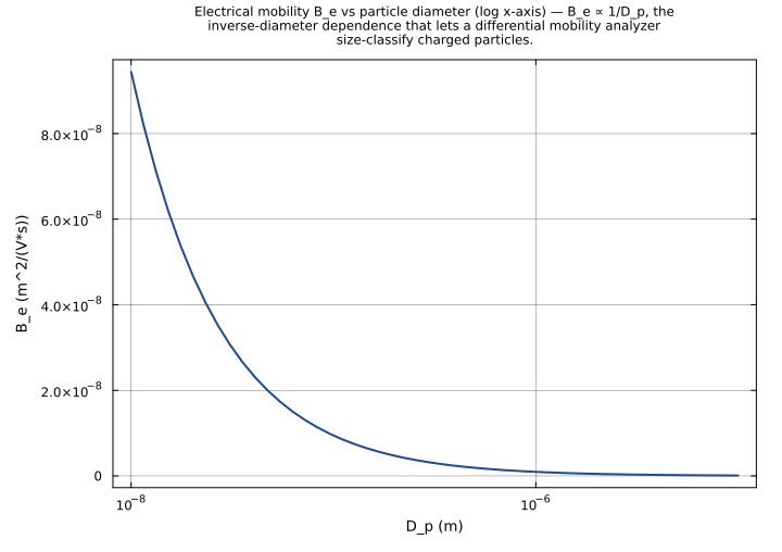
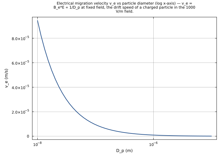
Sweep particle diameter D_p from 10 nm to 10 μm (log scale) at the default single charge (n_charges = 1) and field (E = 1000 V/m). The electrical mobility B_e ∝ 1/D_p falls by three decades across the range, from ≈ 9.4e-8 to ≈ 9.4e-11 m²/(V·s) — smaller particles are far more mobile in an electric field, the principle behind differential mobility analysis. The migration velocity v_e = B_e·E follows the same 1/D_p decline.
Time span: 0.0 → 1.0
Swept over: D_p
Raw .esm
Raw .esm JSON (this component)
{
  "reference": {
    "notes": "source_ref: Aerosol.jl@c8c640bb636b22f2425460e9ed5cba50793bfee1:src/single_particle_dynamics.jl:273\nUpstream `ElectricalMobility` is an MTK `@component` with two constants (π_val, e), five `@parameters` (D_p, μ, C_c, n_charges, E) and three variables (q, B_e, v_e). The equations are:\n  • q   ~ n_charges * e                     (particle charge)\n  • B_e ~ (q * C_c) / (3 * π_val * μ * D_p)  (Eq. 9.50 — electrical mobility)\n  • v_e ~ B_e * E                           (Eq. 9.51 — electrical migration velocity)\nAll three equations are algebraic (no derivatives), making this an observed-only component.\n\nObservability classification: observed-only — every output is given by a single algebraic equation in which the output appears only on the LHS. q is an intermediate algebraic variable: it is the LHS of the charge equation and is reused on the RHS of the B_e equation; B_e is likewise reused on the RHS of the v_e equation, forming a triangular algebraic system. All three outputs migrate as `type: state` with explicit `equations`, matching the sibling single_particle_dynamics.jl migrations mean_free_path.esm, slip.esm, stokes.esm and aerodynamic_diameter.esm (in stokes.esm the intermediate τ is likewise a `type: state` reused by the s_p and St equations). Test scenarios use `time_span: [0, 1]` and sample at t=0.\n\nConstants π_val (3.141592653589793) and e (elementary charge, 1.602e-19 C) migrate as `type: parameter` carrying their numeric defaults, consistent with the sibling single_particle_dynamics.jl migrations (π_val is a `type: parameter` in mean_free_path.esm; the reference-density constant ρ_p0 is a `type: parameter` in aerodynamic_diameter.esm). The name `e` is not one of the ESS schema's reserved physical-constant names (R, k_B, N_A), so it is preserved verbatim from the source.\n\nAll five `@parameters` and both constants appear in the equations, so `parameters(sys)` collects the full set — no unused-parameter pruning is needed.\n\nTolerance rationale (model-level rel=1e-9): observed-only algebraic system (no ODE integration); the q equation is a product of parameters, the B_e equation is a product/division of parameters and q (with π in the denominator), and the v_e equation is a product of B_e and a parameter. Expected values are computed in float64 with the same arithmetic; floating-point round-off is ~1e-15. 1e-9 leaves comfortable headroom."
  },
  "tolerance": {
    "rel": 1e-09
  },
  "variables": {
    "π_val": {
      "type": "parameter",
      "units": "1",
      "default": 3.141592653589793,
      "description": "Pi (dimensionless)"
    },
    "e": {
      "type": "parameter",
      "units": "C",
      "default": 1.602e-19,
      "description": "Elementary charge"
    },
    "D_p": {
      "type": "parameter",
      "units": "m",
      "default": 1e-06,
      "description": "Particle diameter"
    },
    "μ": {
      "type": "parameter",
      "units": "kg/(m*s)",
      "default": 1.8e-05,
      "description": "Dynamic viscosity of air"
    },
    "C_c": {
      "type": "parameter",
      "units": "1",
      "default": 1.0,
      "description": "Slip correction factor (dimensionless)"
    },
    "n_charges": {
      "type": "parameter",
      "units": "1",
      "default": 1.0,
      "description": "Number of elementary charges (dimensionless)"
    },
    "E": {
      "type": "parameter",
      "units": "V/m",
      "default": 1000.0,
      "description": "Electric field strength"
    },
    "q": {
      "type": "unknown",
      "units": "C",
      "description": "Particle charge"
    },
    "B_e": {
      "type": "unknown",
      "units": "m^2/(V*s)",
      "description": "Electrical mobility"
    },
    "v_e": {
      "type": "unknown",
      "units": "m/s",
      "description": "Electrical migration velocity"
    }
  },
  "equations": [
    {
      "lhs": "q",
      "rhs": {
        "op": "*",
        "args": [
          "n_charges",
          "e"
        ]
      }
    },
    {
      "lhs": "B_e",
      "rhs": {
        "op": "/",
        "args": [
          {
            "op": "*",
            "args": [
              "q",
              "C_c"
            ]
          },
          {
            "op": "*",
            "args": [
              {
                "op": "*",
                "args": [
                  {
                    "op": "*",
                    "args": [
                      3,
                      "π_val"
                    ]
                  },
                  "μ"
                ]
              },
              "D_p"
            ]
          }
        ]
      }
    },
    {
      "lhs": "v_e",
      "rhs": {
        "op": "*",
        "args": [
          "B_e",
          "E"
        ]
      }
    }
  ],
  "tests": [
    {
      "id": "default_conditions",
      "description": "Default conditions: D_p = 1.0e-6 m, μ = 1.8e-5 kg/(m·s), C_c = 1.0, n_charges = 1, E = 1000 V/m. A singly-charged particle carries q = n_charges*e = 1.602e-19 C. The electrical mobility B_e = q*C_c/(3π μ D_p) ≈ 9.4432e-10 m²/(V·s), and the migration velocity v_e = B_e*E ≈ 9.4432e-7 m/s.",
      "time_span": {
        "start": 0.0,
        "end": 1.0
      },
      "assertions": [
        {
          "variable": "q",
          "time": 0.0,
          "expected": 1.602e-19
        },
        {
          "variable": "B_e",
          "time": 0.0,
          "expected": 9.443193290119123e-10
        },
        {
          "variable": "v_e",
          "time": 0.0,
          "expected": 9.443193290119123e-07
        }
      ]
    },
    {
      "id": "strong_field",
      "description": "Stronger electric field (E = 5000 V/m) at default particle size and charge: q and B_e are unchanged, but the migration velocity scales linearly with the field, v_e = B_e*E ≈ 4.7216e-6 m/s — five times the default-field value. Mirrors the upstream `v_e = B_e*E` test.",
      "parameter_overrides": {
        "E": 5000.0
      },
      "time_span": {
        "start": 0.0,
        "end": 1.0
      },
      "assertions": [
        {
          "variable": "q",
          "time": 0.0,
          "expected": 1.602e-19
        },
        {
          "variable": "B_e",
          "time": 0.0,
          "expected": 9.443193290119123e-10
        },
        {
          "variable": "v_e",
          "time": 0.0,
          "expected": 4.721596645059562e-06
        }
      ]
    },
    {
      "id": "multiply_charged",
      "description": "Triply-charged particle (n_charges = 3) at default size and field: the charge q = n_charges*e = 4.806e-19 C triples, and because B_e ∝ q the electrical mobility and migration velocity triple as well — B_e ≈ 2.8330e-9 m²/(V·s), v_e ≈ 2.8330e-6 m/s.",
      "parameter_overrides": {
        "n_charges": 3.0
      },
      "time_span": {
        "start": 0.0,
        "end": 1.0
      },
      "assertions": [
        {
          "variable": "q",
          "time": 0.0,
          "expected": 4.806e-19
        },
        {
          "variable": "B_e",
          "time": 0.0,
          "expected": 2.8329579870357367e-09
        },
        {
          "variable": "v_e",
          "time": 0.0,
          "expected": 2.8329579870357367e-06
        }
      ]
    },
    {
      "id": "large_particle",
      "description": "Large particle (D_p = 1.0e-5 m = 10 μm): the charge q is unchanged at 1.602e-19 C, but B_e ∝ 1/D_p, so a 10× larger diameter lowers the electrical mobility 10× to ≈ 9.4432e-11 m²/(V·s) and the migration velocity to ≈ 9.4432e-8 m/s.",
      "parameter_overrides": {
        "D_p": 1e-05
      },
      "time_span": {
        "start": 0.0,
        "end": 1.0
      },
      "assertions": [
        {
          "variable": "q",
          "time": 0.0,
          "expected": 1.602e-19
        },
        {
          "variable": "B_e",
          "time": 0.0,
          "expected": 9.443193290119122e-11
        },
        {
          "variable": "v_e",
          "time": 0.0,
          "expected": 9.443193290119123e-08
        }
      ]
    },
    {
      "id": "small_particle",
      "description": "Small particle (D_p = 1.0e-7 m = 100 nm): B_e ∝ 1/D_p, so a 10× smaller diameter raises the electrical mobility 10× to ≈ 9.4432e-9 m²/(V·s) and the migration velocity to ≈ 9.4432e-6 m/s — small particles respond more strongly to an electric field.",
      "parameter_overrides": {
        "D_p": 1e-07
      },
      "time_span": {
        "start": 0.0,
        "end": 1.0
      },
      "assertions": [
        {
          "variable": "q",
          "time": 0.0,
          "expected": 1.602e-19
        },
        {
          "variable": "B_e",
          "time": 0.0,
          "expected": 9.443193290119123e-09
        },
        {
          "variable": "v_e",
          "time": 0.0,
          "expected": 9.443193290119124e-06
        }
      ]
    },
    {
      "id": "high_slip_correction",
      "description": "Slip correction above unity (C_c = 1.5) at default particle size: B_e ∝ C_c, so a 50% larger slip correction raises the electrical mobility by 50% to ≈ 1.4165e-9 m²/(V·s) and the migration velocity to ≈ 1.4165e-6 m/s. The charge q is unaffected.",
      "parameter_overrides": {
        "C_c": 1.5
      },
      "time_span": {
        "start": 0.0,
        "end": 1.0
      },
      "assertions": [
        {
          "variable": "q",
          "time": 0.0,
          "expected": 1.602e-19
        },
        {
          "variable": "B_e",
          "time": 0.0,
          "expected": 1.4164789935178683e-09
        },
        {
          "variable": "v_e",
          "time": 0.0,
          "expected": 1.4164789935178684e-06
        }
      ]
    }
  ],
  "analyses": [
    {
      "id": "size_dependence",
      "description": "Sweep particle diameter D_p from 10 nm to 10 μm (log scale) at the default single charge (n_charges = 1) and field (E = 1000 V/m). The electrical mobility B_e ∝ 1/D_p falls by three decades across the range, from ≈ 9.4e-8 to ≈ 9.4e-11 m²/(V·s) — smaller particles are far more mobile in an electric field, the principle behind differential mobility analysis. The migration velocity v_e = B_e·E follows the same 1/D_p decline.",
      "initial_state": {},
      "time_span": {
        "start": 0.0,
        "end": 1.0
      },
      "parameter_sweep": {
        "type": "cartesian",
        "dimensions": [
          {
            "parameter": "D_p",
            "range": {
              "start": 1e-08,
              "stop": 1e-05,
              "count": 50,
              "scale": "log"
            }
          }
        ]
      },
      "plots": [
        {
          "id": "mobility_vs_diameter",
          "type": "line",
          "description": "Electrical mobility B_e vs particle diameter (log x-axis) — B_e ∝ 1/D_p, the inverse-diameter dependence that lets a differential mobility analyzer size-classify charged particles.",
          "x": {
            "variable": "D_p",
            "label": "D_p (m)"
          },
          "y": {
            "variable": "B_e",
            "label": "B_e (m^2/(V*s))"
          }
        },
        {
          "id": "migration_velocity_vs_diameter",
          "type": "line",
          "description": "Electrical migration velocity v_e vs particle diameter (log x-axis) — v_e = B_e*E ∝ 1/D_p at fixed field, the drift speed of a charged particle in the 1000 V/m field.",
          "x": {
            "variable": "D_p",
            "label": "D_p (m)"
          },
          "y": {
            "variable": "v_e",
            "label": "v_e (m/s)"
          }
        }
      ]
    }
  ]
}